Note
Go to the end to download the full example code.
Formations
You can plot formations (e.g. 4-4-2) on any mplsoccer pitch using the formation method.
The formations work is a collaboration between
Dmitry Mogilevsky and
Andy Rowlinson.
The formations can be plotted as various options by using the kind argument:
kind='scatter'kind='image'kind='axes'kind='pitch'kind='text'
import math
from urllib.request import urlopen, Request

import matplotlib as mpl
import matplotlib.patheffects as path_effects
import matplotlib.pyplot as plt
import pandas as pd
from PIL import Image

from mplsoccer import VerticalPitch, Sbopen, FontManager, inset_image

# data parser, fonts and path effects for giving the font an edge
parser = Sbopen()
roboto_bold = FontManager(
    'https://raw.githubusercontent.com/google/fonts/main/apache/robotoslab/RobotoSlab%5Bwght%5D.ttf')
path_eff = [path_effects.Stroke(linewidth=3, foreground='white'),
            path_effects.Normal()]
Load StatsBomb data
Load the Starting XI and pass receptions for a Barcelona vs. Real Madrid match for plotting Barcelona’s starting formation.
parser = Sbopen()
event, related, freeze, tactics = parser.event(69249)
# starting players from Barcelona
starting_xi_event = event.loc[((event['type_name'] == 'Starting XI') &
                               (event['team_name'] == 'Barcelona')), ['id', 'tactics_formation']]
# joining on the team name and formation to the lineup
starting_xi = tactics.merge(starting_xi_event, on='id')
# replace player names with the shorter version
player_short_names = {'Víctor Valdés Arribas': 'Víctor Valdés',
                      'Daniel Alves da Silva': 'Dani Alves',
                      'Gerard Piqué Bernabéu': 'Gerard Piqué',
                      'Carles Puyol i Saforcada': 'Carles Puyol',
                      'Eric-Sylvain Bilal Abidal': 'Eric Abidal',
                      'Gnégnéri Yaya Touré': 'Yaya Touré',
                      'Andrés Iniesta Luján': 'Andrés Iniesta',
                      'Xavier Hernández Creus': 'Xavier Hernández',
                      'Lionel Andrés Messi Cuccittini': 'Lionel Messi',
                      'Thierry Henry': 'Thierry Henry',
                      "Samuel Eto''o Fils": "Samuel Eto'o"}
starting_xi['player_name'] = starting_xi['player_name'].replace(player_short_names)
# filter only succesful ball receipts from the starting XI
event = event.loc[((event['type_name'] == 'Ball Receipt') &
                   (event['outcome_name'].isnull()) &
                   (event['player_id'].isin(starting_xi['player_id']))
                   ), ['player_id', 'x', 'y']]
# merge on the starting positions to the events
event = event.merge(starting_xi, on='player_id')
formation = event['tactics_formation'].iloc[0]
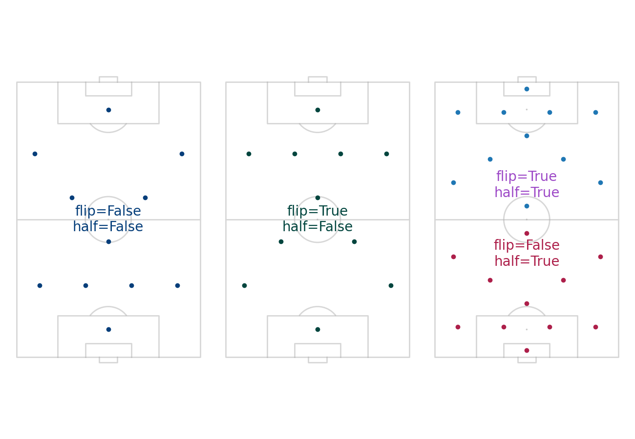
Flip and half
You can plot the formations in different configurations using the flip and half arguments.
pitch = VerticalPitch(line_alpha=0.5, goal_type='box', goal_alpha=0.5)
fig, ax = pitch.draw(ncols=3, figsize=(13, 9))
sc_full = pitch.formation(formation, positions=starting_xi.position_id, c='#053e7a', ax=ax[0])
sc_flip = pitch.formation(formation, positions=starting_xi.position_id, c='#01453e', flip=True,
                          ax=ax[1])
sc_half = pitch.formation(formation, positions=starting_xi.position_id, c='#ad1f4a', half=True,
                          ax=ax[2])
sc_half_flip = pitch.formation(formation, positions=starting_xi.position_id, kind='scatter',
                               flip=True, half=True, ax=ax[2])

txt_full = pitch.text(60, 40, 'flip=False\nhalf=False', ax=ax[0], va='center', ha='center',
                      color='#053e7a', fontsize=20)
txt_flip = pitch.text(60, 40, 'flip=True\nhalf=False', ax=ax[1], va='center', ha='center',
                      color='#01453e', fontsize=20)
txt_half = pitch.text(45, 40, 'flip=False\nhalf=True', ax=ax[2], va='center', ha='center',
                      color='#ad1f4a', fontsize=20)
txt_half_flip = pitch.text(75, 40, 'flip=True\nhalf=True', ax=ax[2], va='center', ha='center',
                           color='#9d49c7', fontsize=20)
Get images
Let’s get some images from Wikipedia. Note, it would be better if these all had the same aspect ratio for plotting.
image_urls = {
    # Credit: Darz Mol. Creative Commons Attribution-Share Alike 2.5 Spain license.
    # https://en.wikipedia.org/wiki/V%C3%ADctor_Vald%C3%A9s#/media/File:Victor_Valdes_15abr2007.jpg
    'Víctor Valdés': 'https://upload.wikimedia.org/wikipedia/commons/4/46/Victor_Valdes_15abr2007.jpg',
    # Credit: Football.ua. CC BY-SA 3.0
    # https://en.wikipedia.org/wiki/Dani_Alves#/media/File:2015_UEFA_Super_Cup_107.jpg
    'Dani Alves': 'https://upload.wikimedia.org/wikipedia/commons/1/1f/2015_UEFA_Super_Cup_107.jpg',
    # Credit: Shay. CC BY-SA 3.0
    # https://en.wikipedia.org/wiki/Gerard_Piqu%C3%A9#/media/File:Gerard_Pique.jpg
    'Gerard Piqué': 'https://upload.wikimedia.org/wikipedia/commons/e/e1/Gerard_Pique.jpg',
    # Credit: Shay. CC BY-SA 3.0
    # https://en.wikipedia.org/wiki/Carles_Puyol#/media/File:Carles_Puyol_Joan_Gamper-Tr.jpg
    'Carles Puyol': 'https://upload.wikimedia.org/wikipedia/commons/6/60/Carles_Puyol_Joan_Gamper-Tr.jpg',
    # Credit: Mutari. Public Domain
    # https://en.wikipedia.org/wiki/Eric_Abidal#/media/File:%C3%89ric_Abidal_-_001.jpg
    'Eric Abidal': 'https://upload.wikimedia.org/wikipedia/commons/c/c8/%C3%89ric_Abidal_-_001.jpg',
    # Credit: Football.ua. CC BY-SA 3.0
    # https://en.wikipedia.org/wiki/Yaya_Tour%C3%A9#/media/File:Yaya_Tour%C3%A9.JPG
    'Yaya Touré': 'https://upload.wikimedia.org/wikipedia/commons/e/ee/Yaya_Tour%C3%A9.JPG',
    # Credit: Darz Mol CC BY-SA 2.5 es
    # https://en.wikipedia.org/wiki/Andr%C3%A9s_Iniesta#/media/File:Andr%C3%A9s_Iniesta_21dec2006.jpg
    'Andrés Iniesta': 'https://upload.wikimedia.org/wikipedia/commons/e/ed/Andr%C3%A9s_Iniesta_21dec2006.jpg',
    # Credit: Castroquini. CC BY-SA 3.0
    # https://en.wikipedia.org/wiki/Xavi#/media/File:2012_2013_-_06_Xavi_Hern%C3%A1ndez.jpg
    'Xavier Hernández': 'https://upload.wikimedia.org/wikipedia/commons/9/93/2012_2013_-_06_Xavi_Hern%C3%A1ndez.jpg',
    # Credit: Tasnim News Agency. CC BY 4.0
    # https://fi.wikipedia.org/wiki/Lionel_Messi#/media/Tiedosto:Lionel-Messi-Argentina-2022-FIFA-World-Cup_(cropped).jpg
    'Lionel Messi': 'https://upload.wikimedia.org/wikipedia/commons/b/b4/Lionel-Messi-Argentina-2022-FIFA-World-Cup_%28cropped%29.jpg',
    # Credit: Shay. CC BY-SA 3.0
    # https://en.wikipedia.org/wiki/Thierry_Henry#/media/File:Thierry_Henry_2008.jpg
    'Thierry Henry': 'https://upload.wikimedia.org/wikipedia/commons/6/6e/Thierry_Henry_2008.jpg',
    # Credit: Shay. CC BY-SA 3.0
    # https://en.wikipedia.org/wiki/Samuel_Eto%27o#/media/File:Etoo_Joan_Gamper_Trophy_2008.jpg
    "Samuel Eto'o": 'https://upload.wikimedia.org/wikipedia/commons/7/77/Etoo_Joan_Gamper_Trophy_2008.jpg',
}
images = []
for url in starting_xi.player_name.map(image_urls):
    request = Request(url)
    request.add_header('User-Agent', 'mplsoccerdocs (https://mplsoccer.rtfd.io)')
    images.append(Image.open(urlopen(request)))
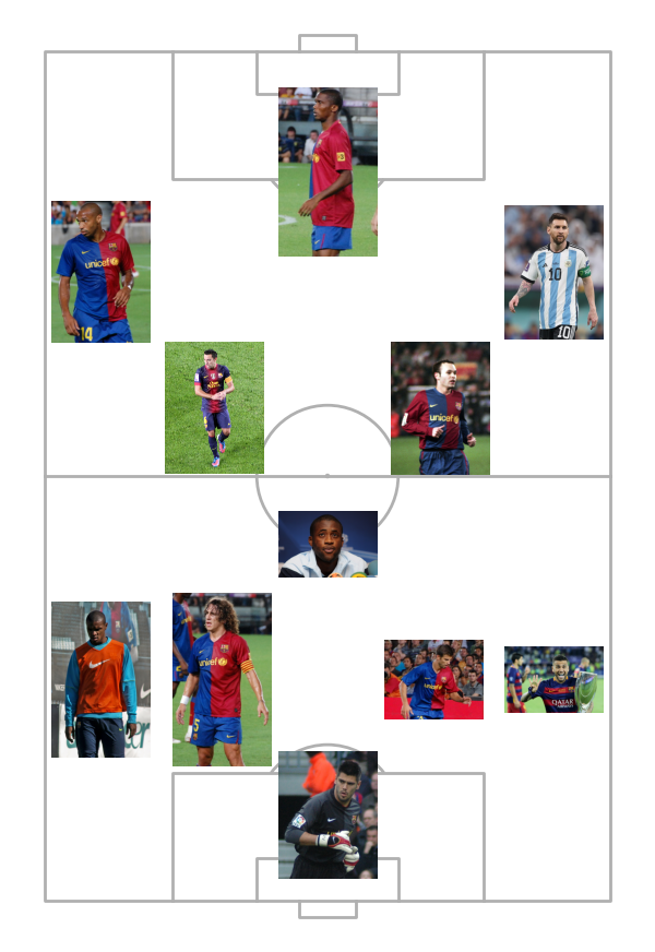
Formation of images
You can plot the formations as images using kind='image' and image arguments.
Here we use xoffset and yoffset to eliminate some overlapping images.
The offsets should be in the same order as the positions argument (i.e. player identifiers).
Additional keyword arguments are passed on to Axes.imshow.
pitch = VerticalPitch(goal_type='box')
fig, ax = pitch.draw(figsize=(6, 8.72))
ax_image = pitch.formation(formation, positions=starting_xi.position_id, kind='image', image=images,
                           width=14,
                           xoffset=[0, 0, 0, 0, 0, 0, 0, 0, 0, 0, -5],
                           # xoffset in same order as the positions
                           yoffset=[0, 2, 5, -5, -2, 0, 0, 0, 0, 0, 0],
                           # yoffset in the same order as the positions
                           ax=ax)
# comment below sets this as the thumbnail in the docs
# sphinx_gallery_thumbnail_path = 'gallery/pitch_plots/images/sphx_glr_plot_formations_002'
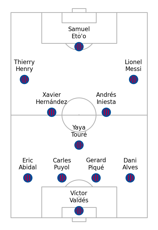
Text and scatter
You can plot the formations as text using kind='text' and the text arguments.
Additional keyword arguments are passed on to Axes.text.
Here we also plot kind='scatter' to add a marker for each position and additional
arguments are passed on to Axes.scatter.
pitch = VerticalPitch(goal_type='box')
fig, ax = pitch.draw(figsize=(6, 8.72))
ax_text = pitch.formation(formation, positions=starting_xi.position_id, kind='text',
                          text=starting_xi.player_name.str.replace(' ', '\n'),
                          va='center', ha='center', fontsize=16, ax=ax)
# scatter markers
mpl.rcParams['hatch.linewidth'] = 3
mpl.rcParams['hatch.color'] = '#a50044'
ax_scatter = pitch.formation(formation, positions=starting_xi.position_id, kind='scatter',
                             c='#004d98', hatch='||', linewidth=3, s=500,
                             # you can also provide a single offset instead of a list
                             # for xoffset and yoffset
                             xoffset=-8,
                             ax=ax)
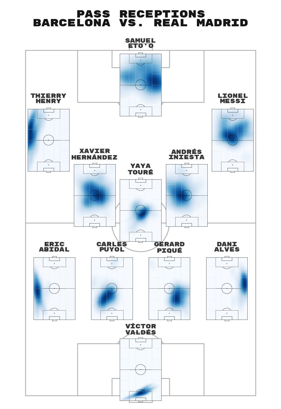
Pitch of pitches
You can plot the formations as pitches using the kind='pitch' argument.
I believe UtdArena was the first
person to introduce this type of visualization.
Additional keyword arguments amend the inset pitch’s appearance, e.g. line_color.
In this example, it is the first game that Messi played as a false-nine. After around 7 minutes Eto’o” and Messi switched positions, which is why their heatmaps look the wrong way around.
pitch = VerticalPitch(goal_type='box')
fig, axs = pitch.grid(endnote_height=0, title_height=0.08, figheight=14, grid_width=0.9,
                      grid_height=0.9, axis=False)
fm_rubik = FontManager('https://raw.githubusercontent.com/google/fonts/main/ofl/'
                       'rubikmonoone/RubikMonoOne-Regular.ttf')
title = axs['title'].text(0.5, 0.5, 'Pass receptions\nBarcelona vs. Real Madrid', fontsize=25,
                          va='center',
                          ha='center', color='#161616', fontproperties=fm_rubik.prop)

pitch_ax = pitch.formation(formation,
                           kind='pitch',
                           # avoid overlapping pitches with offsets
                           xoffset=[-3, 6, 6, 6, 6, 14, 0, 0, 0, 0, 0],
                           # pitch is 23 units long (could also set the height).
                           # note this is set assuming the pitch is horizontal, but in this example
                           # it is vertical so that you get the same results
                           # from both VerticalPitch and Pitch
                           width=23,
                           positions=starting_xi['position_id'],
                           ax=axs['pitch'],
                           # additional arguments temporarily amend the pitch appearance
                           # note we are plotting a really faint positional grid
                           # that overlays the kdeplot
                           linewidth=0.5,
                           pitch_color='None',
                           line_zorder=3,
                           line_color='black',
                           positional=True,
                           positional_zorder=3,
                           positional_linewidth=1,
                           positional_alpha=0.3,
                           )

# adding kdeplot and player titles
for position in pitch_ax:
    player_name = starting_xi[starting_xi['position_id'] == position].player_name.iloc[0]
    player_name = player_name.replace(' ', '\n').replace('-', '-\n')
    pitch.text(150, 40, player_name, va='top', ha='center', fontsize=15, ax=pitch_ax[position],
               fontproperties=fm_rubik.prop, color='#353535')
    pitch.kdeplot(x=event.loc[event['position_id'] == position, 'x'],
                  y=event.loc[event['position_id'] == position, 'y'],
                  fill=True, levels=100, cut=100, cmap='Blues', thresh=0, ax=pitch_ax[position])
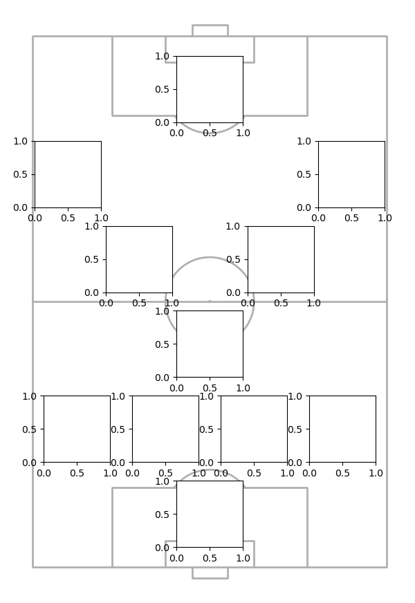
Axes
You can plot the formation as axes. Additional keyword arguments are passed on to Axes.inset_axes.
pitch = VerticalPitch(goal_type='box')
fig, ax = pitch.draw(figsize=(6, 8.72))
ax_text = pitch.formation(formation, positions=starting_xi.position_id, height=15, aspect=1,
                          kind='axes', ax=ax)
Get Opta data
mplsoccer also supports Wyscout and Opta formations. Let’s generate some data for the Team of the Week using Opta’s position identifiers. We will use the ‘4-3-3’ formation.
Note, all the Opta formations are included in mplsoccer. However, ‘412112’ could be called ‘4-4-2 diamond’ in Opta’s data and ‘31213’ could be called ‘343’ in Opta’s data.
totw_player_data = pd.DataFrame(
    {
        'position': ['LW', 'ST', 'RW', 'LCM', 'CDM', 'RCM', 'LB', 'LCB', 'RCB', 'RB', 'GK'],
        'position_id': [11, 9, 10, 8, 4, 7, 3, 6, 5, 2, 1],
        'player': ['Reiten', 'Kerr', 'Fleming', 'Charles', 'Miedema', 'Kirby', 'Blundell',
                   'Greenwood', 'Bryson', 'Battle', 'Earps'],
        'score': [9.7, 8.6, 8.7, 9.1, 8.7, 9.5, 7.6, 8.0, 8.0, 9.1, 8.3],
        'team': ['Chelsea', 'Chelsea', 'Chelsea', 'Chelsea', 'Arsenal', 'Chelsea',
                 'Manchester United', 'Manchester City', 'Reading', 'Manchester United',
                 'Manchester United']
    }
)
totw_player_data
Get the club badges as a dictionary and turn it into a list of badges for each player.
badge_urls = {
    'Manchester United': 'https://upload.wikimedia.org/wikipedia/en/thumb/7/7a/Manchester_United_FC_crest.svg/250px-Manchester_United_FC_crest.svg.png',
    'Chelsea': 'https://upload.wikimedia.org/wikipedia/en/thumb/c/cc/Chelsea_FC.svg/250px-Chelsea_FC.svg.png',
    'Manchester City': 'https://upload.wikimedia.org/wikipedia/en/thumb/e/eb/Manchester_City_FC_badge.svg/250px-Manchester_City_FC_badge.svg.png',
    'Reading': 'https://upload.wikimedia.org/wikipedia/en/thumb/1/11/Reading_FC.svg/250px-Reading_FC.svg.png',
    'Arsenal': "https://upload.wikimedia.org/wikipedia/en/thumb/5/53/Arsenal_FC.svg/250px-Arsenal_FC.svg.png",
}
image_dict = {}
for team, url in badge_urls.items():
    request = Request(url)
    request.add_header('User-Agent', 'mplsoccerdocs (https://mplsoccer.rtfd.io)')
    image_dict[team] = Image.open(urlopen(request))
images = [image_dict[team] for team in totw_player_data.team]
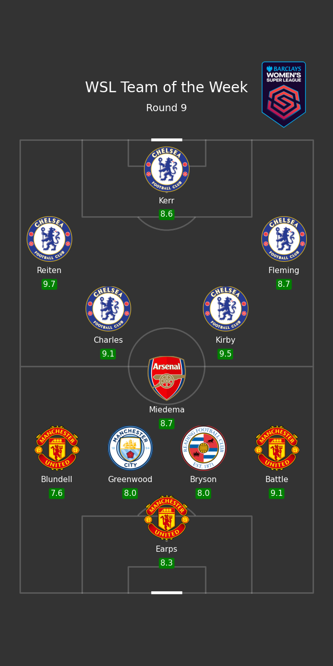
Plotting Opta data
Next, create the pitch figure using pitch.grid to create a header space for the title.
We use the formation method to create text and images for each position in the formation
and use xoffsets to adjust the positions to avoid overlaps
# setup figure
pitch = VerticalPitch(pitch_type='opta', pitch_color='#333333', line_color='white', line_alpha=0.2,
                      line_zorder=3)
fig, axes = pitch.grid(endnote_height=0, figheight=13, title_height=0.1, title_space=0, space=0)
fig.set_facecolor('#333333')

# title
axes['title'].axis('off')
axes['title'].text(0.5, 0.6, 'WSL Team of the Week', ha='center', va='center', color='white',
                   fontsize=20)
axes['title'].text(0.5, 0.3, 'Round 9', ha='center', va='center', color='white', fontsize=14)
text_names = pitch.formation('433', kind='text', positions=totw_player_data.position_id,
                             text=totw_player_data.player, ax=axes['pitch'],
                             xoffset=-2,  # offset the player names from the centers
                             ha='center', va='center', color='white', fontsize=11)
text_scores = pitch.formation('433', kind='text', positions=totw_player_data.position_id,
                              text=totw_player_data.score, ax=axes['pitch'],
                              xoffset=-5,  # offset the scores from the centers
                              ha='center', va='center', color='white', fontsize=11,
                              bbox=dict(facecolor='green', boxstyle='round,pad=0.2', linewidth=0))
badge_axes = pitch.formation('433', kind='image', positions=totw_player_data.position_id,
                             image=images, height=10, ax=axes['pitch'],
                             xoffset=5,  # offset the images from the centers
                             )
Get Wyscout data
The next example uses some example Wyscout data.
wyscout_data = {'player_name': ['David de Gea', 'Bailly', 'Maguire', 'Shaw',
                                'Wan-Bissaka', 'Matić', 'Fred', 'Williams',
                                'Bruno Fernandes', 'James', 'Martial'],
                'position_id': ['gk', 'rcb3', 'cb', 'lcb3', 'rwb', 'rcmf', 'lcmf', 'lwb', 'amf',
                                'ss', 'cf'],
                }
WYSCOUT_FORMATION = '3-4-1-2'
df_wyscout = pd.DataFrame(wyscout_data)
df_wyscout
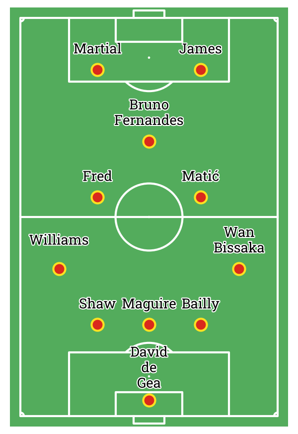
Plotting Wyscout formations
Here we plot the ‘3-4-1-2’ formation on a Wyscout pitch. Note for some formations in the Wyscout data there are two attacking midfielders (‘amf’) In mplsoccer, we have assigned the right position ‘ramf’ and the left position ‘lamf’. You may have to arbitrarily assign your ‘amf’ positions to these positions.
pitch = VerticalPitch(pitch_type='wyscout', goal_type='box', pitch_color='#53ac5c',
                      line_color='white', linewidth=3, corner_arcs=True)
fig, ax = pitch.draw(figsize=(6, 8.72))
sc_formation = pitch.formation(WYSCOUT_FORMATION, positions=wyscout_data['position_id'],
                               ax=ax, c='#DA291C', ec='#FBE122',
                               xoffset=[-6, -3, -3, -3, -5, -3, -3, -5, -5, -3, -3],
                               yoffset=[0, 0, 0, 0, -5, 0, 0, 5, 0, 0, 0],
                               lw=3, s=300)
sc_text = pitch.formation(WYSCOUT_FORMATION, positions=wyscout_data['position_id'],
                          text=df_wyscout['player_name'].str.replace(' ', '\n').str.replace('-',
                                                                                            '\n'),
                          yoffset=[0, 0, 0, 0, -5, 0, 0, 5, 0, 0, 0],
                          kind='text', va='center', ha='center', xoffset=2,
                          fontsize=20, fontproperties=roboto_bold.prop, path_effects=path_eff,
                          ax=ax)
Valid formations
You can print a list of the valid formations included in mplsoccer. mplsoccer also accepts the hyphenated versions and the Wyscout formations that include zeros, e.g. ‘4-4-2’ and ‘5-3-0’.
pitch = VerticalPitch()
print(pitch.formations)
['442', '41212', '433', '451', '4411', '4141', '4231', '4321', '532', '541', '352', '532flat', '343', '343flat', '31312', '4222', '3511', '3511flat', '3421', '3421flat', '3412', '3412flat', '3142', '31213', '4132', '424', '4312', '3241', '3331', 'pyramid', 'metodo', 'wm', '41221', '42211', '32221', '5221', '3232', '312112', '42121', '31222', '4213', '32122', '3322', '41131', '432', '441', '4311', '4221', '4131', '4212', '342', '3411', '351', '531', '431', '44', '422', '341', '53', '1234', '1324', '1432', '1423', '2422', '2413', '2431', '2332', '2233']
Valid positions
You can also return a dataframe of the formations, positions and coordinates.
pitch.formations_dataframe
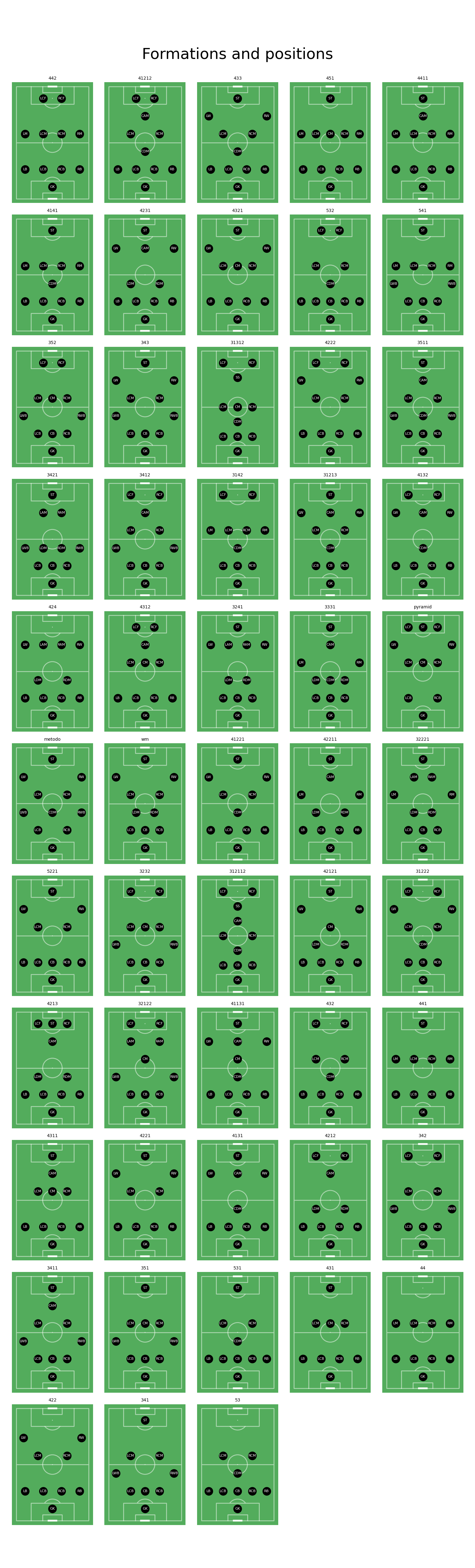
Available formations
Below is a showcase of all available formations and their positions.
pitch = VerticalPitch('uefa', line_alpha=0.5, pitch_color='#53ac5c', line_color='white')

df_formations = pitch.formations_dataframe
COLS = 5
rows = math.ceil(len(pitch.formations) / COLS)

fig, axes = pitch.grid(nrows=rows, ncols=COLS, title_height=0.015, endnote_height=0, figheight=50,
                       space=0.08, grid_height=0.92)
axes_p = axes['pitch'].flatten()
for i, formation in enumerate(pitch.formations):
    pitch.formation(formation, kind='scatter', color='black', s=350, ax=axes_p[i])
    pitch.formation(formation, kind='text',
                    positions=df_formations.loc[df_formations.formation == formation, 'name'],
                    text=df_formations.loc[df_formations.formation == formation, 'name'],
                    color='white', fontsize=8, ha='center', va='center', ax=axes_p[i])
    axes_p[i].set_title(formation, fontsize=10)
axes['title'].axis('off')
title = axes['title'].text(0.5, 0.5, 'Formations and positions', fontsize=35,
                           ha='center', va='center')

# remove spare axes
number_spare_axes = (COLS * rows) - len(pitch.formations)
for j in range(1, number_spare_axes + 1):
    axes_p[-j].remove()
Positions dataframe
If you want to access the underlying positions. You can do this with the get_positions
method. There are four variations with either four or five positions in each line,
line=4 or line=5, and either second_striker=True or second_striker=False.
The positions without a second striker have more space around the attacking positions.
pitch.get_positions(line=5, second_striker=True)
plt.show() # If you are using a Jupyter notebook you do not need this line
Total running time of the script: (0 minutes 9.953 seconds)