Pitch Basics

First we import the Pitch classes and matplotlib

import matplotlib.pyplot as plt

from mplsoccer import Pitch, VerticalPitch

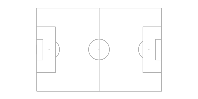
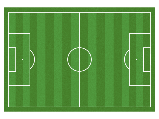
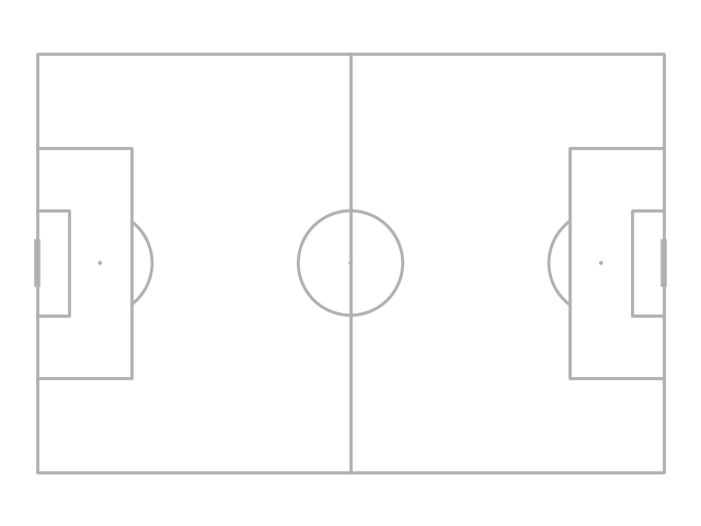
Draw a pitch on a new axis

Let’s plot on a new axis first.

pitch = Pitch()
# specifying figure size (width, height)
fig, ax = pitch.draw(figsize=(8, 4))

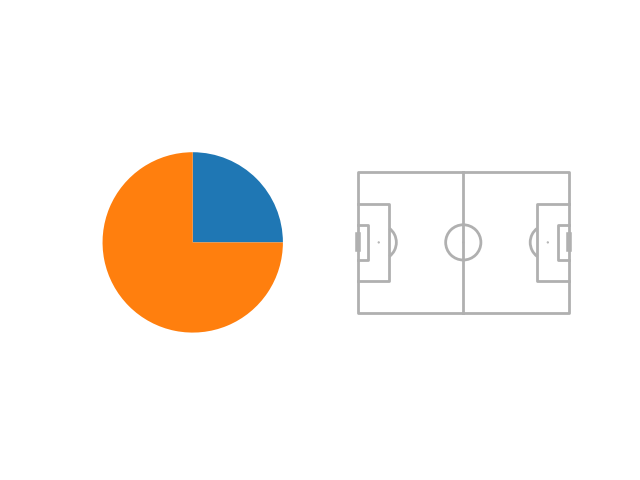
Draw on an existing axis

mplsoccer also plays nicely with other matplotlib figures. To draw a pitch on an existing matplotlib axis specify an ax in the draw method.

fig, axs = plt.subplots(nrows=1, ncols=2)
pitch = Pitch()
pie = axs[0].pie(x=[5, 15])
pitch.draw(ax=axs[1])

Supported data providers

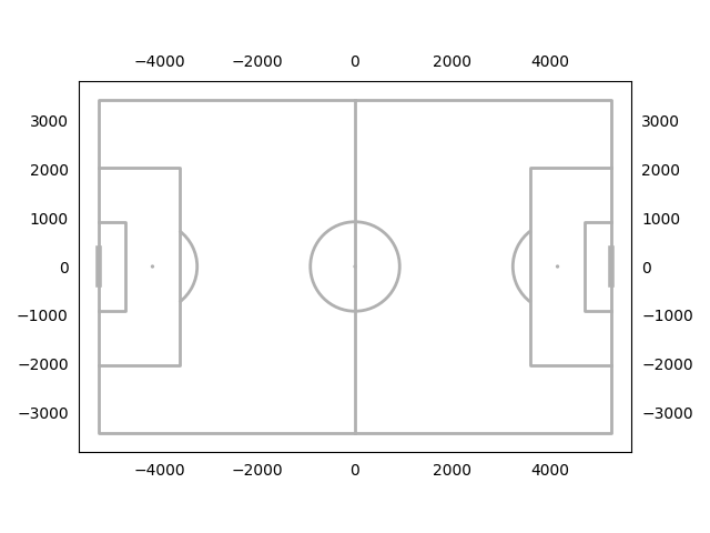
mplsoccer supports 10 pitch types by specifying the pitch_type argument: ‘statsbomb’, ‘opta’, ‘tracab’, ‘wyscout’, ‘uefa’, ‘metricasports’, ‘custom’, ‘skillcorner’, ‘secondspectrum’ and ‘impect’. If you are using tracking data or the custom pitch (‘metricasports’, ‘tracab’, ‘skillcorner’, ‘secondspectrum’ or ‘custom’), you also need to specify the pitch_length and pitch_width, which are typically 105 and 68 respectively.

pitch = Pitch(pitch_type='opta')  # example plotting an Opta/ Stats Perform pitch
fig, ax = pitch.draw()

pitch = Pitch(pitch_type='tracab',  # example plotting a tracab pitch
              pitch_length=105, pitch_width=68,
              axis=True, label=True)  # showing axis labels is optional
fig, ax = pitch.draw()

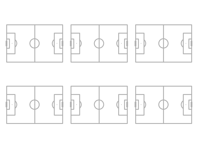
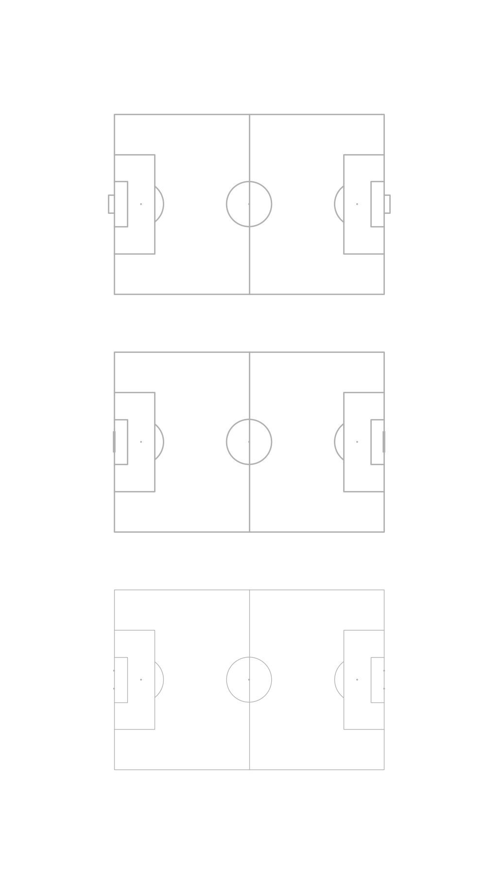
Adjusting the plot layout

mplsoccer also plots on grids by specifying nrows and ncols. The default is to use tight_layout. See: https://matplotlib.org/stable/tutorials/intermediate/tight_layout_guide.html.

pitch = Pitch()
fig, axs = pitch.draw(nrows=2, ncols=3)

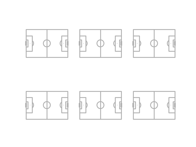
But you can also use constrained layout by setting constrained_layout=True and tight_layout=False, which may look better. See: https://matplotlib.org/stable/tutorials/intermediate/constrainedlayout_guide.html.

pitch = Pitch()
fig, axs = pitch.draw(nrows=2, ncols=3, tight_layout=False, constrained_layout=True)

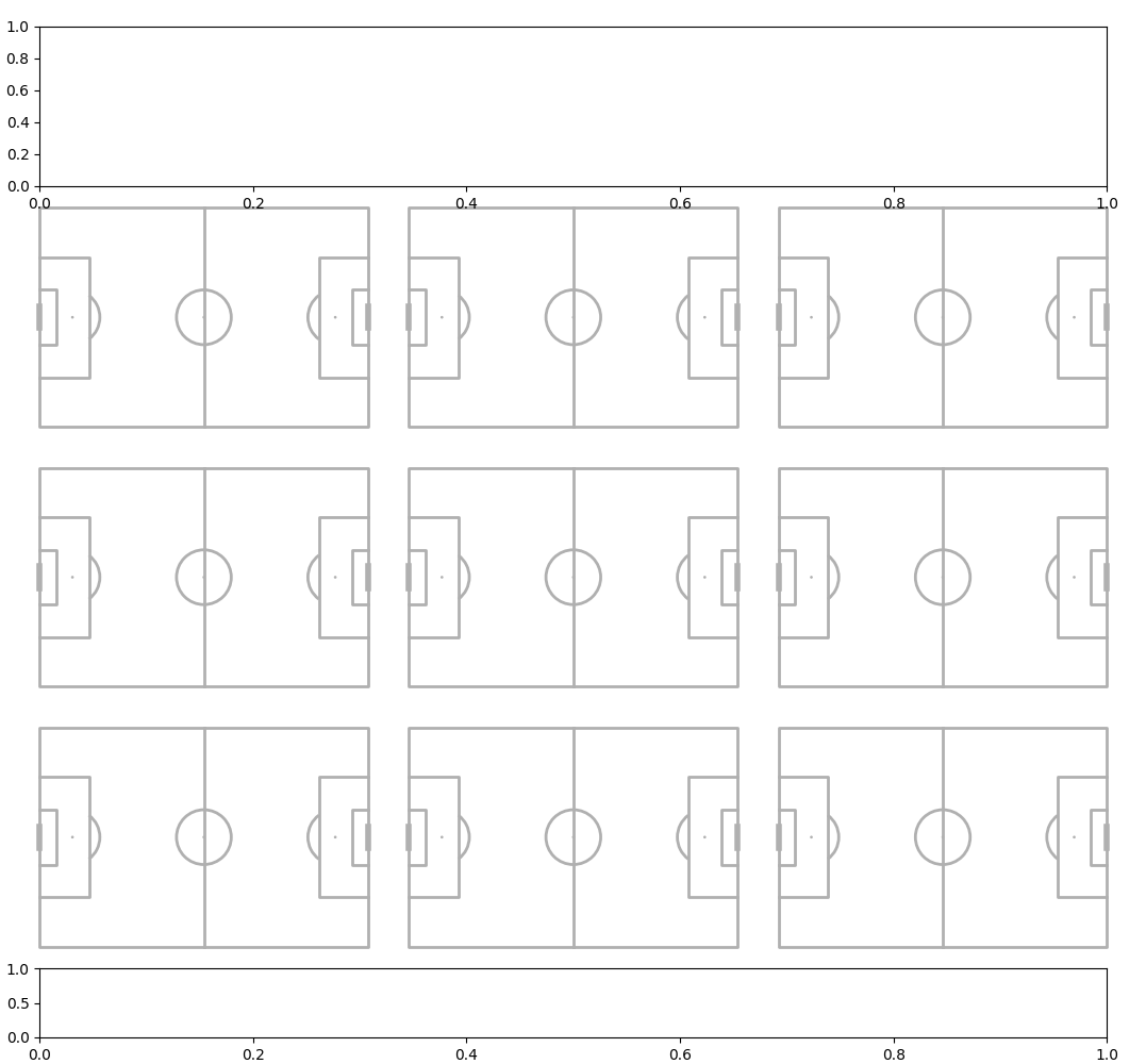
If you want more control over how pitches are placed you can use the grid method. This also works for one pitch (nrows=1 and ncols=1). It also plots axes for an endnote and title (see the plot_grid example for more information).

pitch = Pitch()
fig, axs = pitch.grid(nrows=3, ncols=3, figheight=10,
                      # the grid takes up 71.5% of the figure height
                      grid_height=0.715,
                      # 5% of grid_height is reserved for space between axes
                      space=0.05,
                      # centers the grid horizontally / vertically
                      left=None, bottom=None)

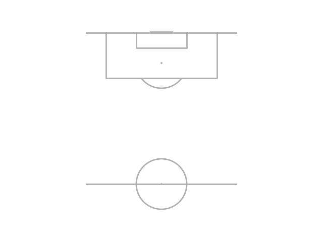
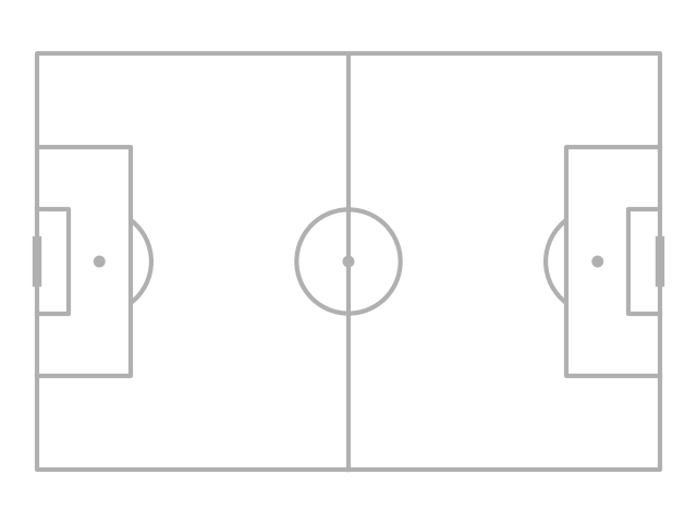
Pitch orientation

There are four basic pitch orientations. To get vertical pitches use the VerticalPitch class. To get half pitches use the half=True argument.

Horizontal full

pitch = Pitch(half=False)
fig, ax = pitch.draw()

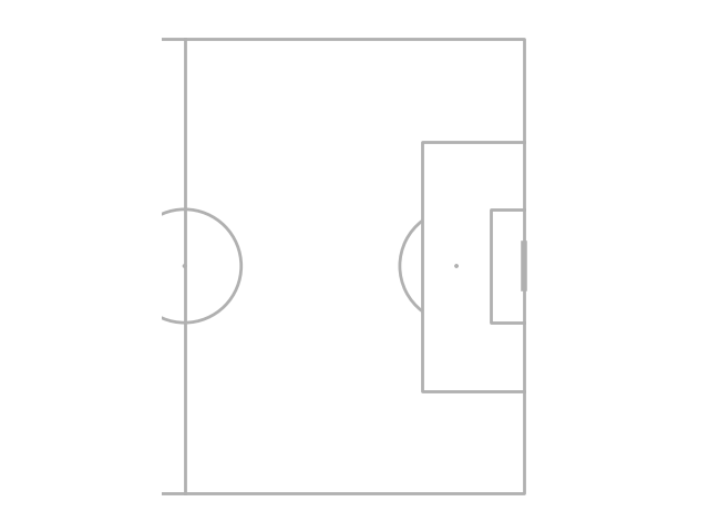
Vertical full

pitch = VerticalPitch(half=False)
fig, ax = pitch.draw()

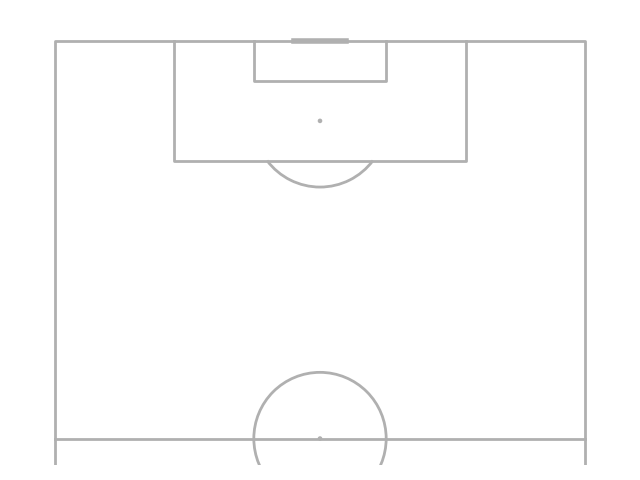
Horizontal half

pitch = Pitch(half=True)
fig, ax = pitch.draw()

Vertical half

pitch = VerticalPitch(half=True)
fig, ax = pitch.draw()

You can also adjust the pitch orientations with the pad_left, pad_right, pad_bottom and pad_top arguments to make arbitrary pitch shapes.

pitch = VerticalPitch(half=True,
                      pad_left=-10,  # bring the left axis in 10 data units (reduce the size)
                      pad_right=-10,  # bring the right axis in 10 data units (reduce the size)
                      pad_top=10,  # extend the top axis 10 data units
                      pad_bottom=20)  # extend the bottom axis 20 data units
fig, ax = pitch.draw()

Pitch appearance

The pitch appearance is adjustable. Use pitch_color and line_color, and stripe_color (if stripe=True) to adjust the colors.

pitch = Pitch(pitch_color='#aabb97', line_color='white',
              stripe_color='#c2d59d', stripe=True)  # optional stripes
fig, ax = pitch.draw()

Line style

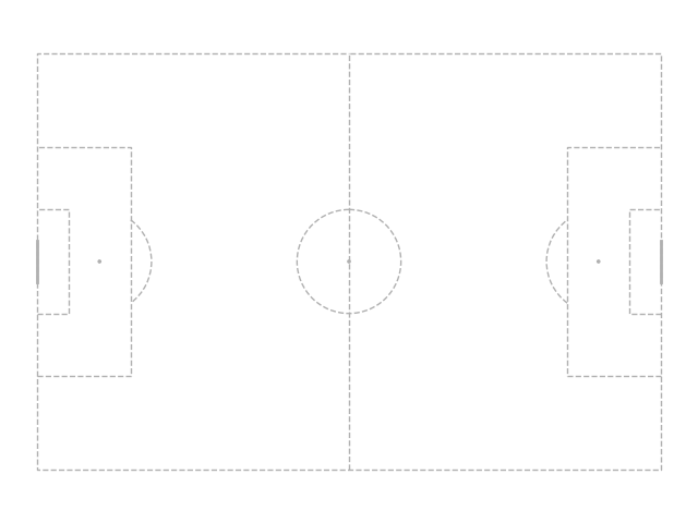
The pitch line style is adjustable. Use linestyle and goal_linestyle to adjust the colors.

pitch = Pitch(linestyle='--', linewidth=1, goal_linestyle='-')
fig, ax = pitch.draw()

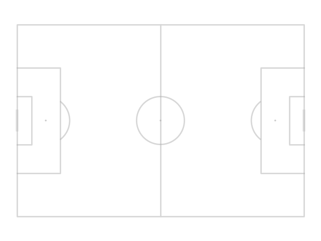
Line alpha

The pitch transparency is adjustable. Use pitch_alpha and goal_alpha to adjust the colors.

pitch = Pitch(line_alpha=0.5, goal_alpha=0.3)
fig, ax = pitch.draw()

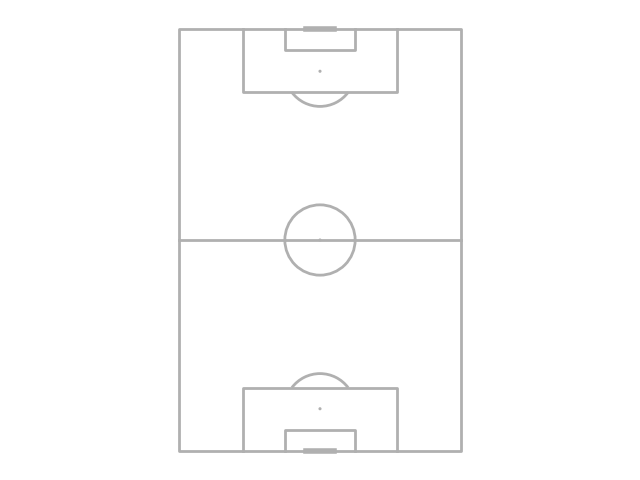
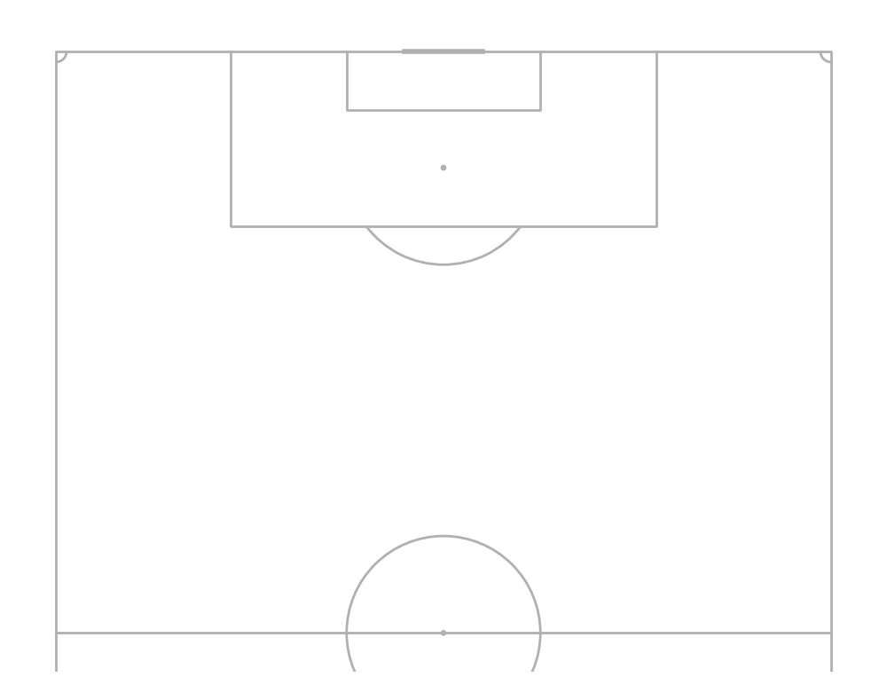
Corner arcs

You can add corner arcs to the pitch by setting corner_arcs = True

pitch = VerticalPitch(corner_arcs=True, half=True)
fig, ax = pitch.draw(figsize=(10, 7.727))

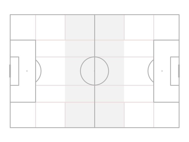
Juego de Posición

You can add the Juego de Posición pitch lines and shade the middle third. You can also adjust the transparency via shade_alpha and positional_alpha.

pitch = Pitch(positional=True, shade_middle=True, positional_color='#eadddd', shade_color='#f2f2f2')
fig, ax = pitch.draw()

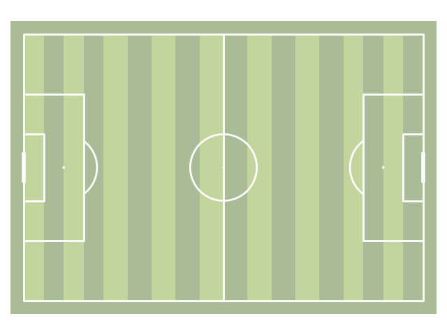
mplsoccer can also plot grass pitches by setting pitch_color='grass'.

pitch = Pitch(pitch_color='grass', line_color='white',
              stripe=True)  # optional stripes
fig, ax = pitch.draw()

Three goal types are included goal_type='line', goal_type='box', and goal_type='circle'

fig, axs = plt.subplots(nrows=3, figsize=(10, 18))
pitch = Pitch(goal_type='box', goal_alpha=1)  # you can also adjust the transparency (alpha)
pitch.draw(axs[0])
pitch = Pitch(goal_type='line')
pitch.draw(axs[1])
pitch = Pitch(goal_type='circle', linewidth=1)
pitch.draw(axs[2])

The line markings and spot size can be adjusted via linewidth and spot_scale. Spot scale also adjusts the size of the circle goal posts.

pitch = Pitch(linewidth=3,
              # the size of the penalty and center spots relative to the pitch_length
              spot_scale=0.01)
fig, ax = pitch.draw()

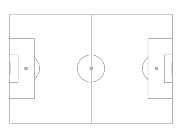
The center and penalty spots can also be changed to a square to avoid clashes with scatter points.

pitch = Pitch(spot_type='square', spot_scale=0.01)
fig, ax = pitch.draw()

If you need to lift the pitch markings above other elements of the chart. You can do this via line_zorder, stripe_zorder, positional_zorder, and shade_zorder.

pitch = Pitch(line_zorder=2)  # e.g. useful if you want to plot pitch lines over heatmaps
fig, ax = pitch.draw()

Axis

By default mplsoccer turns of the axis (border), ticks, and labels. You can use them by setting the axis, label and tick arguments.

pitch = Pitch(axis=True, label=True, tick=True)
fig, ax = pitch.draw()

xkcd

Finally let’s use matplotlib’s xkcd theme.

plt.xkcd()
pitch = Pitch(pitch_color='grass', stripe=True)
fig, ax = pitch.draw(figsize=(8, 4))
annotation = ax.annotate('Who can resist this?', (60, 10), fontsize=30, ha='center')

plt.show()  # If you are using a Jupyter notebook you do not need this line