Note
Go to the end to download the full example code.
Radar Charts
mplsoccer,radar_chartmodule helps one to plot radar charts in a few lines of code.The radar-chart inspiration is StatsBomb and Rami Moghadam
Here we will show some examples of how to use
mplsoccerto plot radar charts.
We have re-written the Soccerplots Radar module to enable greater customisation of the Radar. You can now set the edge color, decide the number of concentric circles, and use hatching or path_effects.
from mplsoccer import Radar, FontManager, grid
import matplotlib.pyplot as plt
Setting the Radar Boundaries
One of the most important decisions with Radars is setting the Radar’s boundaries. StatsBomb popularised the use of Radars for showing player statistics. I recommend checking out understanding football radars for mugs and muggles. StatsBomb’s rule of thumb is: “Radar boundaries represent the top 5% and bottom 5% of all statistical production by players in that position.”
# parameter names of the statistics we want to show
params = ["npxG", "Non-Penalty Goals", "xA", "Key Passes", "Through Balls",
          "Progressive Passes", "Shot-Creating Actions", "Goal-Creating Actions",
          "Dribbles Completed", "Pressure Regains", "Touches In Box", "Miscontrol"]

# The lower and upper boundaries for the statistics
low =  [0.08, 0.0, 0.1, 1, 0.6,  4, 3, 0.3, 0.3, 2.0, 2, 0]
high = [0.37, 0.6, 0.6, 4, 1.2, 10, 8, 1.3, 1.5, 5.5, 5, 5]

# Add anything to this list where having a lower number is better
# this flips the statistic
lower_is_better = ['Miscontrol']
Instantiate the Radar Class
We will instantiate a Radar object with the above parameters so that we can re-use it
several times.
radar = Radar(params, low, high,
              lower_is_better=lower_is_better,
              # whether to round any of the labels to integers instead of decimal places
              round_int=[False]*len(params),
              num_rings=4,  # the number of concentric circles (excluding center circle)
              # if the ring_width is more than the center_circle_radius then
              # the center circle radius will be wider than the width of the concentric circles
              ring_width=1, center_circle_radius=1)
Load some fonts
We will use mplsoccer’s FontManager to load some fonts from Google Fonts.
We borrowed the FontManager from the excellent
ridge_map library.
URL1 = ('https://raw.githubusercontent.com/googlefonts/SourceSerifProGFVersion/main/fonts/'
        'SourceSerifPro-Regular.ttf')
serif_regular = FontManager(URL1)
URL2 = ('https://raw.githubusercontent.com/googlefonts/SourceSerifProGFVersion/main/fonts/'
        'SourceSerifPro-ExtraLight.ttf')
serif_extra_light = FontManager(URL2)
URL3 = ('https://raw.githubusercontent.com/google/fonts/main/ofl/rubikmonoone/'
        'RubikMonoOne-Regular.ttf')
rubik_regular = FontManager(URL3)
URL4 = 'https://raw.githubusercontent.com/googlefonts/roboto/main/src/hinted/Roboto-Thin.ttf'
robotto_thin = FontManager(URL4)
URL5 = ('https://raw.githubusercontent.com/google/fonts/main/apache/robotoslab/'
        'RobotoSlab%5Bwght%5D.ttf')
robotto_bold = FontManager(URL5)
Player Values
Here are the player values we are going to plot. The values are taken from the excellent fbref website (supplied by StatsBomb).
bruno_values =   [0.22, 0.25, 0.30, 2.54, 0.43, 5.60, 4.34, 0.29, 0.69, 5.14, 4.97, 1.10]
bruyne_values =  [0.25, 0.52, 0.37, 3.59, 0.41, 6.36, 5.68, 0.57, 1.23, 4.00, 4.54, 1.39]
erikson_values = [0.13, 0.10, 0.35, 3.08, 0.29, 6.23, 5.08, 0.43, 0.67, 3.07, 1.34, 1.06]
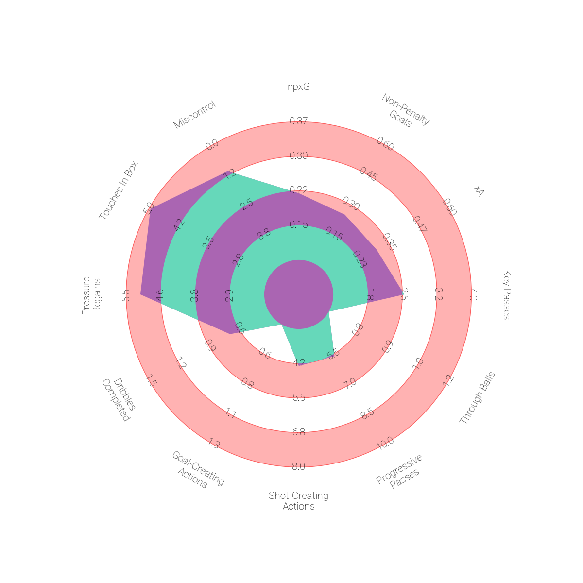
Making a Simple Radar Chart
Here we will make a very simple radar chart using the radar_chart module.
We will only change the default face and edge colors.
fig, ax = radar.setup_axis()  # format axis as a radar
rings_inner = radar.draw_circles(ax=ax, facecolor='#ffb2b2', edgecolor='#fc5f5f')  # draw circles
radar_output = radar.draw_radar(bruno_values, ax=ax,
                                kwargs_radar={'facecolor': '#aa65b2'},
                                kwargs_rings={'facecolor': '#66d8ba'})  # draw the radar
radar_poly, rings_outer, vertices = radar_output
range_labels = radar.draw_range_labels(ax=ax, fontsize=15,
                                       fontproperties=robotto_thin.prop)  # draw the range labels
param_labels = radar.draw_param_labels(ax=ax, fontsize=15,
                                       fontproperties=robotto_thin.prop)  # draw the param labels
Adding lines from the center to the edge
Here we add spokes from the radar center to the edge using Radar.spoke.
fig, ax = radar.setup_axis()  # format axis as a radar
rings_inner = radar.draw_circles(ax=ax, facecolor='#ffb2b2', edgecolor='#fc5f5f')  # draw circles
radar_output = radar.draw_radar(bruno_values, ax=ax,
                                kwargs_radar={'facecolor': '#aa65b2'},
                                kwargs_rings={'facecolor': '#66d8ba'})  # draw the radar
radar_poly, rings_outer, vertices = radar_output
range_labels = radar.draw_range_labels(ax=ax, fontsize=15, zorder=2.5,
                                       fontproperties=robotto_thin.prop)  # draw the range labels
param_labels = radar.draw_param_labels(ax=ax, fontsize=15,
                                       fontproperties=robotto_thin.prop)  # draw the param labels
lines = radar.spoke(ax=ax, color='#a6a4a1', linestyle='--', zorder=2)

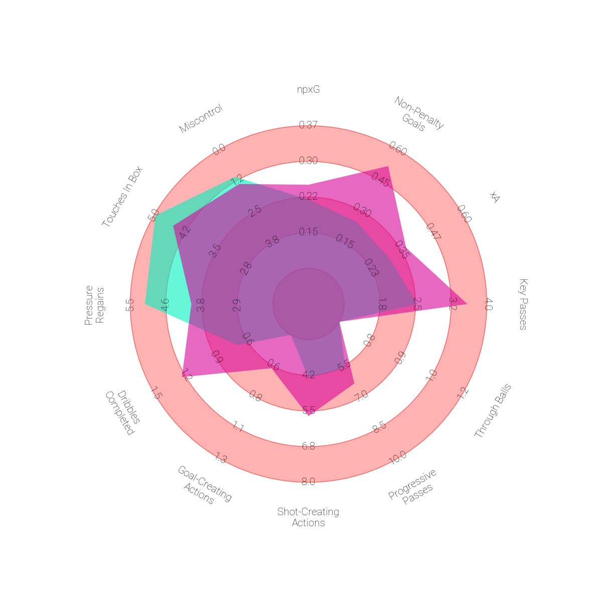
Making a Simple Comparison
Here we plot two players on the same axes to compare players.
# plot radar
fig, ax = radar.setup_axis()
rings_inner = radar.draw_circles(ax=ax, facecolor='#ffb2b2', edgecolor='#fc5f5f')
radar_output = radar.draw_radar_compare(bruno_values, bruyne_values, ax=ax,
                                        kwargs_radar={'facecolor': '#00f2c1', 'alpha': 0.6},
                                        kwargs_compare={'facecolor': '#d80499', 'alpha': 0.6})
radar_poly, radar_poly2, vertices1, vertices2 = radar_output
range_labels = radar.draw_range_labels(ax=ax, fontsize=15,
                                       fontproperties=robotto_thin.prop)
param_labels = radar.draw_param_labels(ax=ax, fontsize=15,
                                       fontproperties=robotto_thin.prop)
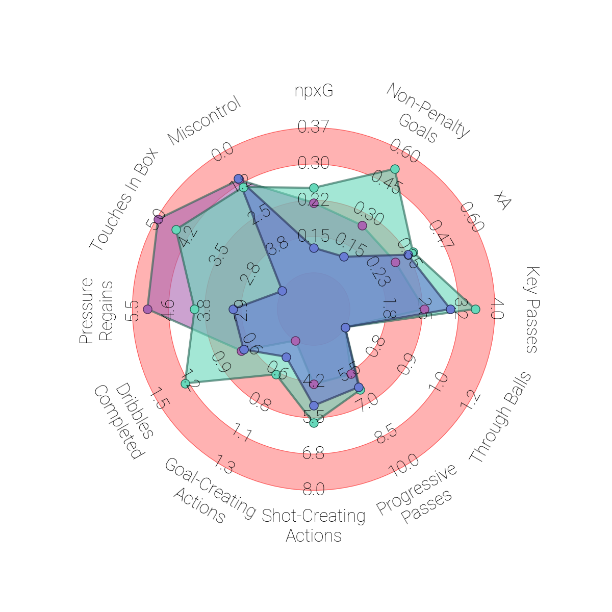
Comparing three or more players
Here we demonstrate comparing three players on the same chart. It’s possible to
add as many as you want by stacking Radar.draw_radar_solid
# plot radar
fig, ax = radar.setup_axis()
rings_inner = radar.draw_circles(ax=ax, facecolor='#ffb2b2', edgecolor='#fc5f5f')

radar1, vertices1 = radar.draw_radar_solid(bruno_values, ax=ax,
                                           kwargs={'facecolor': '#aa65b2',
                                                   'alpha': 0.6,
                                                   'edgecolor': '#216352',
                                                   'lw': 3})

radar2, vertices2 = radar.draw_radar_solid(bruyne_values, ax=ax,
                                           kwargs={'facecolor': '#66d8ba',
                                                   'alpha': 0.6,
                                                   'edgecolor': '#216352',
                                                   'lw': 3})

radar3, vertices3 = radar.draw_radar_solid(erikson_values, ax=ax,
                                           kwargs={'facecolor': '#697cd4',
                                                   'alpha': 0.6,
                                                   'edgecolor': '#222b54',
                                                   'lw': 3})

ax.scatter(vertices1[:, 0], vertices1[:, 1],
           c='#aa65b2', edgecolors='#502a54', marker='o', s=150, zorder=2)
ax.scatter(vertices2[:, 0], vertices2[:, 1],
           c='#66d8ba', edgecolors='#216352', marker='o', s=150, zorder=2)
ax.scatter(vertices3[:, 0], vertices3[:, 1],
           c='#697cd4', edgecolors='#222b54', marker='o', s=150, zorder=2)

range_labels = radar.draw_range_labels(ax=ax, fontsize=25, fontproperties=robotto_thin.prop)
param_labels = radar.draw_param_labels(ax=ax, fontsize=25, fontproperties=robotto_thin.prop)
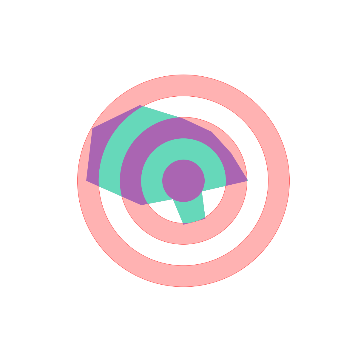
Making a Clean Radar
Here we exclude the label lines from the plot.
fig, ax = radar.setup_axis()  # format axis as a radar
rings_inner = radar.draw_circles(ax=ax, facecolor='#ffb2b2', edgecolor='#fc5f5f')  # draw circles
radar_output = radar.draw_radar(bruno_values, ax=ax,
                                kwargs_radar={'facecolor': '#aa65b2'},
                                kwargs_rings={'facecolor': '#66d8ba'})  # draw the radar
radar_poly, rings_outer, vertices = radar_output
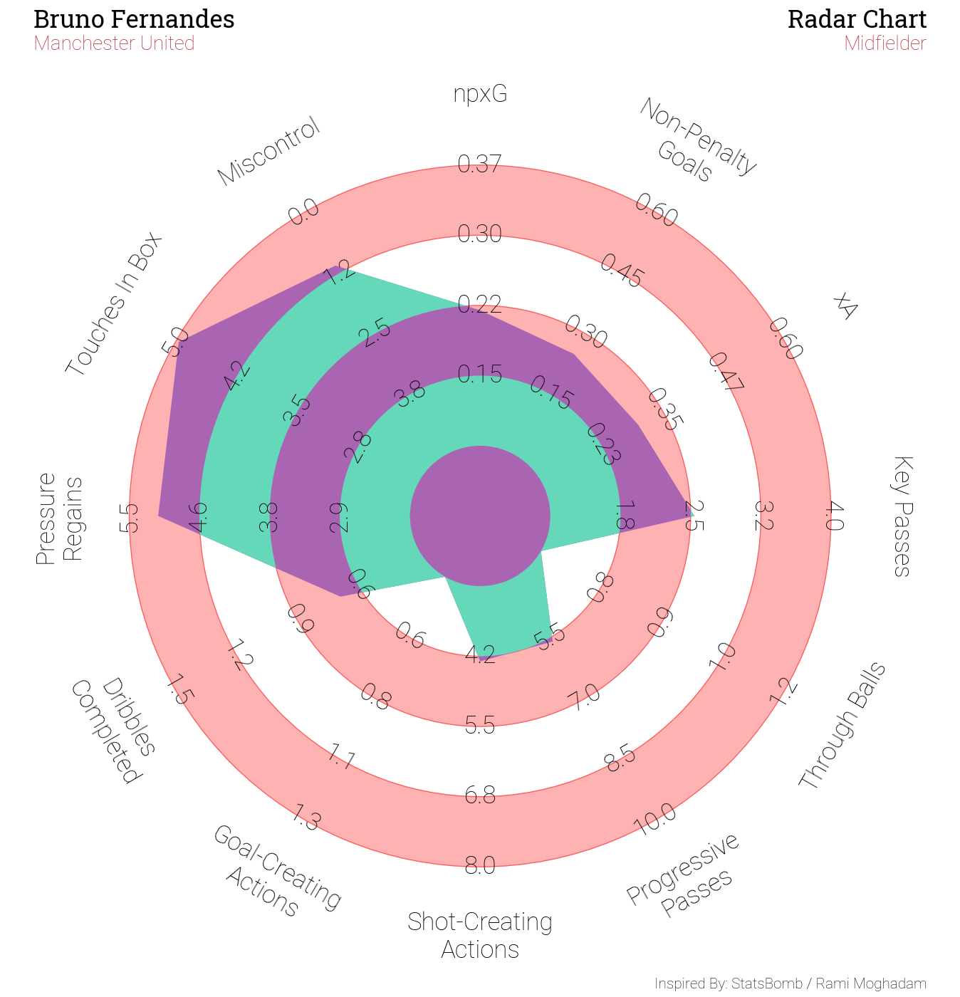
Adding a title and endnote
Here we will add an endnote and title to the Radar. We will use the grid function to create the figure and pass the axs[‘radar’] axes to the Radar’s methods.
# creating the figure using the grid function from mplsoccer:
fig, axs = grid(figheight=14, grid_height=0.915, title_height=0.06, endnote_height=0.025,
                title_space=0, endnote_space=0, grid_key='radar', axis=False)

# plot the radar
radar.setup_axis(ax=axs['radar'])
rings_inner = radar.draw_circles(ax=axs['radar'], facecolor='#ffb2b2', edgecolor='#fc5f5f')
radar_output = radar.draw_radar(bruno_values, ax=axs['radar'],
                                kwargs_radar={'facecolor': '#aa65b2'},
                                kwargs_rings={'facecolor': '#66d8ba'})
radar_poly, rings_outer, vertices = radar_output
range_labels = radar.draw_range_labels(ax=axs['radar'], fontsize=25,
                                       fontproperties=robotto_thin.prop)
param_labels = radar.draw_param_labels(ax=axs['radar'], fontsize=25,
                                       fontproperties=robotto_thin.prop)

# adding the endnote and title text (these axes range from 0-1, i.e. 0, 0 is the bottom left)
# Note we are slightly offsetting the text from the edges by 0.01 (1%, e.g. 0.99)
endnote_text = axs['endnote'].text(0.99, 0.5, 'Inspired By: StatsBomb / Rami Moghadam', fontsize=15,
                                   fontproperties=robotto_thin.prop, ha='right', va='center')
title1_text = axs['title'].text(0.01, 0.65, 'Bruno Fernandes', fontsize=25,
                                fontproperties=robotto_bold.prop, ha='left', va='center')
title2_text = axs['title'].text(0.01, 0.25, 'Manchester United', fontsize=20,
                                fontproperties=robotto_thin.prop,
                                ha='left', va='center', color='#B6282F')
title3_text = axs['title'].text(0.99, 0.65, 'Radar Chart', fontsize=25,
                                fontproperties=robotto_bold.prop, ha='right', va='center')
title4_text = axs['title'].text(0.99, 0.25, 'Midfielder', fontsize=20,
                                fontproperties=robotto_thin.prop,
                                ha='right', va='center', color='#B6282F')
# sphinx_gallery_thumbnail_path = 'gallery/radar/images/sphx_glr_plot_radar_004.png'
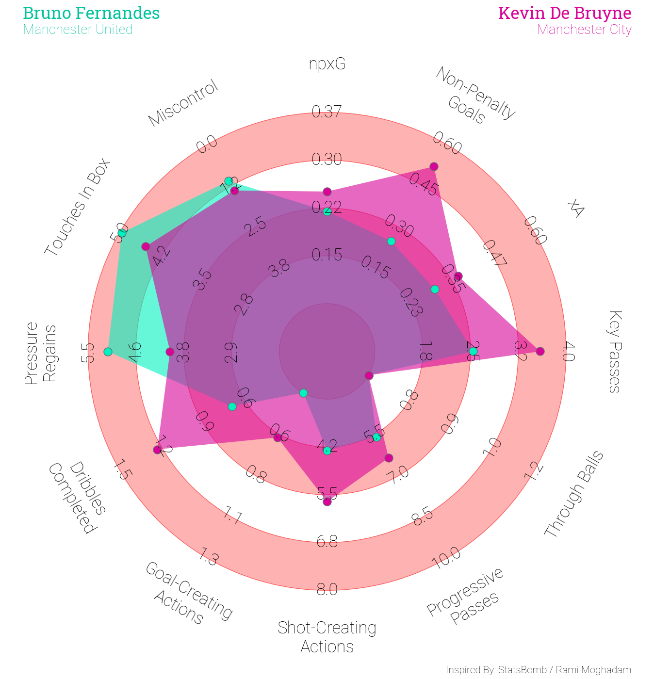
Comparison Radar with Titles
Here we will make a very simple radar chart using mplsoccer module radar_chart.
We will only change the default facecolors.
# creating the figure using the grid function from mplsoccer:
fig, axs = grid(figheight=14, grid_height=0.915, title_height=0.06, endnote_height=0.025,
                title_space=0, endnote_space=0, grid_key='radar', axis=False)

# plot radar
radar.setup_axis(ax=axs['radar'])  # format axis as a radar
rings_inner = radar.draw_circles(ax=axs['radar'], facecolor='#ffb2b2', edgecolor='#fc5f5f')
radar_output = radar.draw_radar_compare(bruno_values, bruyne_values, ax=axs['radar'],
                                        kwargs_radar={'facecolor': '#00f2c1', 'alpha': 0.6},
                                        kwargs_compare={'facecolor': '#d80499', 'alpha': 0.6})
radar_poly, radar_poly2, vertices1, vertices2 = radar_output
range_labels = radar.draw_range_labels(ax=axs['radar'], fontsize=25,
                                       fontproperties=robotto_thin.prop)
param_labels = radar.draw_param_labels(ax=axs['radar'], fontsize=25,
                                       fontproperties=robotto_thin.prop)
axs['radar'].scatter(vertices1[:, 0], vertices1[:, 1],
                     c='#00f2c1', edgecolors='#6d6c6d', marker='o', s=150, zorder=2)
axs['radar'].scatter(vertices2[:, 0], vertices2[:, 1],
                     c='#d80499', edgecolors='#6d6c6d', marker='o', s=150, zorder=2)

# adding the endnote and title text (these axes range from 0-1, i.e. 0, 0 is the bottom left)
# Note we are slightly offsetting the text from the edges by 0.01 (1%, e.g. 0.99)
endnote_text = axs['endnote'].text(0.99, 0.5, 'Inspired By: StatsBomb / Rami Moghadam', fontsize=15,
                                   fontproperties=robotto_thin.prop, ha='right', va='center')
title1_text = axs['title'].text(0.01, 0.65, 'Bruno Fernandes', fontsize=25, color='#01c49d',
                                fontproperties=robotto_bold.prop, ha='left', va='center')
title2_text = axs['title'].text(0.01, 0.25, 'Manchester United', fontsize=20,
                                fontproperties=robotto_thin.prop,
                                ha='left', va='center', color='#01c49d')
title3_text = axs['title'].text(0.99, 0.65, 'Kevin De Bruyne', fontsize=25,
                                fontproperties=robotto_bold.prop,
                                ha='right', va='center', color='#d80499')
title4_text = axs['title'].text(0.99, 0.25, 'Manchester City', fontsize=20,
                                fontproperties=robotto_thin.prop,
                                ha='right', va='center', color='#d80499')
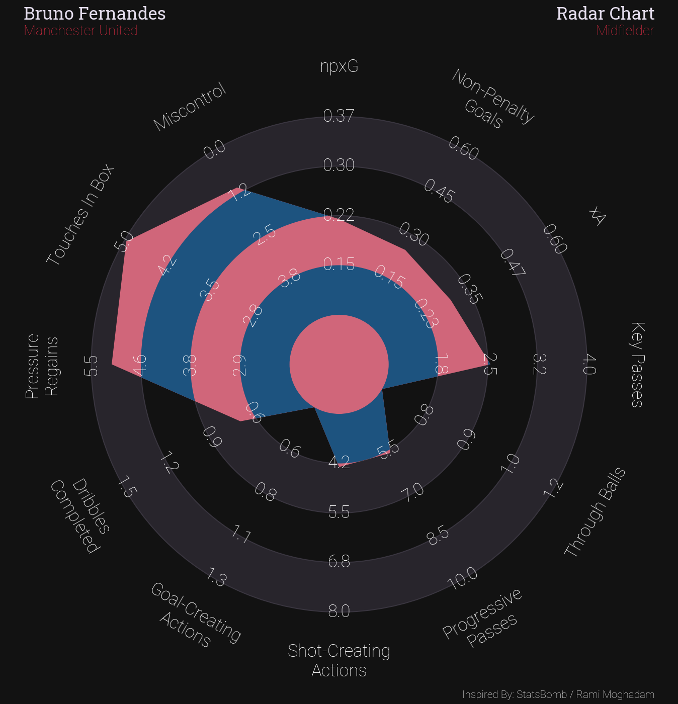
Dark Theme
# creating the figure using the grid function from mplsoccer:
fig, axs = grid(figheight=14, grid_height=0.915, title_height=0.06, endnote_height=0.025,
                title_space=0, endnote_space=0, grid_key='radar', axis=False)

# plot the radar
radar.setup_axis(ax=axs['radar'], facecolor='None')
rings_inner = radar.draw_circles(ax=axs['radar'], facecolor='#28252c', edgecolor='#39353f', lw=1.5)
radar_output = radar.draw_radar(bruno_values, ax=axs['radar'],
                                kwargs_radar={'facecolor': '#d0667a'},
                                kwargs_rings={'facecolor': '#1d537f'})
radar_poly, rings_outer, vertices = radar_output
range_labels = radar.draw_range_labels(ax=axs['radar'], fontsize=25, color='#fcfcfc',
                                       fontproperties=robotto_thin.prop)
param_labels = radar.draw_param_labels(ax=axs['radar'], fontsize=25, color='#fcfcfc',
                                       fontproperties=robotto_thin.prop)

# adding the endnote and title text (these axes range from 0-1, i.e. 0, 0 is the bottom left)
# Note we are slightly offsetting the text from the edges by 0.01 (1%, e.g. 0.99)
endnote_text = axs['endnote'].text(0.99, 0.5, 'Inspired By: StatsBomb / Rami Moghadam',
                                   color='#fcfcfc', fontproperties=robotto_thin.prop,
                                   fontsize=15, ha='right', va='center')
title1_text = axs['title'].text(0.01, 0.65, 'Bruno Fernandes', fontsize=25,
                                fontproperties=robotto_bold.prop,
                                ha='left', va='center', color='#e4dded')
title2_text = axs['title'].text(0.01, 0.25, 'Manchester United', fontsize=20,
                                fontproperties=robotto_thin.prop,
                                ha='left', va='center', color='#cc2a3f')
title3_text = axs['title'].text(0.99, 0.65, 'Radar Chart', fontsize=25,
                                fontproperties=robotto_bold.prop,
                                ha='right', va='center', color='#e4dded')
title4_text = axs['title'].text(0.99, 0.25, 'Midfielder', fontsize=20,
                                fontproperties=robotto_thin.prop,
                                ha='right', va='center', color='#cc2a3f')

fig.set_facecolor('#121212')
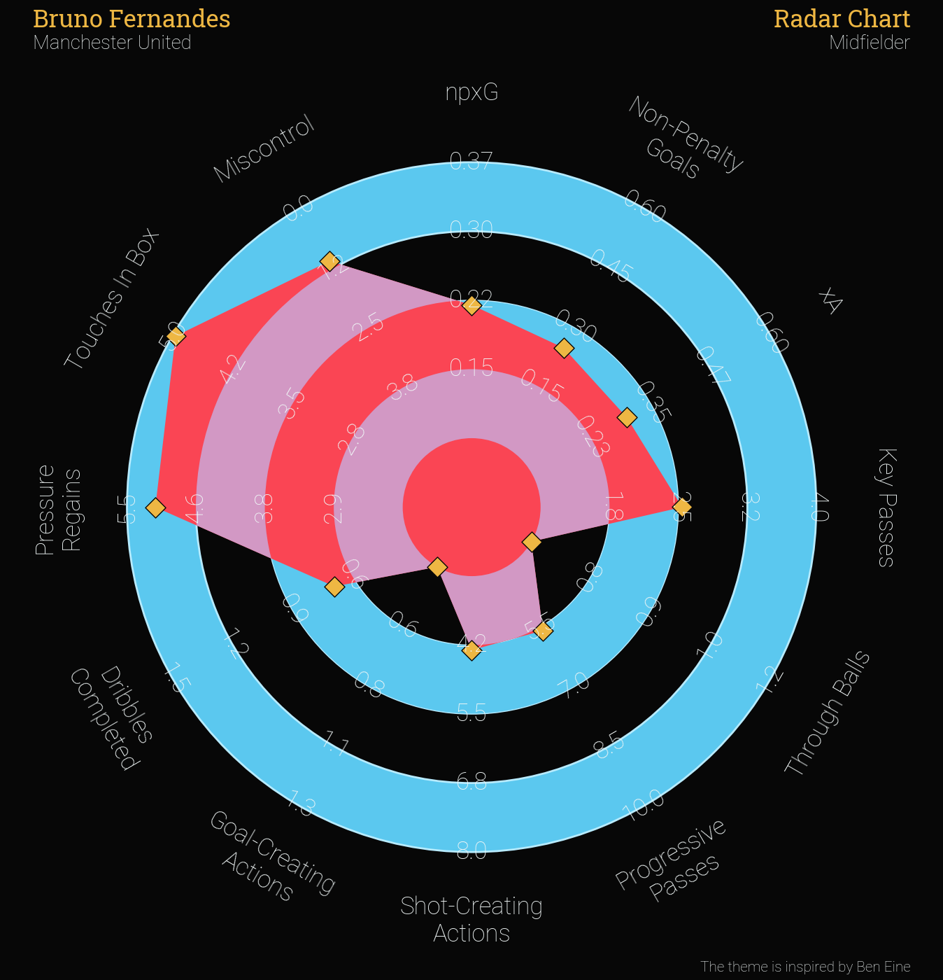
Ben Eine Theme
The theme below is inspired by the artist Ben Eine.
# creating the figure using the grid function from mplsoccer:
fig, axs = grid(figheight=14, grid_height=0.915, title_height=0.06, endnote_height=0.025,
                title_space=0, endnote_space=0, grid_key='radar', axis=False)

# plot the radar
radar.setup_axis(ax=axs['radar'], facecolor='None')
rings_inner = radar.draw_circles(ax=axs['radar'], facecolor='#5bc8ef', edgecolor='#b7ebff',
                                 # you can also vary the linewidths
                                 # here we gradually increase the blue concentric circles
                                 linewidth=[0, 1, 2])
radar_output = radar.draw_radar(bruno_values, ax=axs['radar'],
                                kwargs_radar={'facecolor': '#fa4554'},
                                kwargs_rings={'facecolor': '#d298c4'})
radar_poly, rings_outer, vertices = radar_output
range_labels = radar.draw_range_labels(ax=axs['radar'], fontsize=25, color='#f0f6f6',
                                       fontproperties=robotto_thin.prop)
param_labels = radar.draw_param_labels(ax=axs['radar'], fontsize=25, color='#f0f6f6',
                                       fontproperties=robotto_thin.prop)
axs['radar'].scatter(vertices[:, 0], vertices[:, 1], c='#eeb743', edgecolors='#070707',
                     marker='D', s=220, zorder=2)

# adding the endnote and title text (these axes range from 0-1, i.e. 0, 0 is the bottom left)
# Note we are slightly offsetting the text from the edges by 0.01 (1%, e.g. 0.99)
endnote_text = axs['endnote'].text(0.99, 0.5, 'The theme is inspired by Ben Eine', fontsize=15,
                                   fontproperties=robotto_thin.prop, ha='right',
                                   va='center', color='#f0f6f6')
title1_text = axs['title'].text(0.01, 0.65, 'Bruno Fernandes', fontsize=25,
                                fontproperties=robotto_bold.prop, ha='left',
                                va='center', color='#eeb743')
title2_text = axs['title'].text(0.01, 0.25, 'Manchester United', fontsize=20,
                                fontproperties=robotto_thin.prop, ha='left',
                                va='center', color='#f0f6f6')
title3_text = axs['title'].text(0.99, 0.65, 'Radar Chart', fontsize=25,
                                fontproperties=robotto_bold.prop, ha='right',
                                va='center', color='#eeb743')
title4_text = axs['title'].text(0.99, 0.25, 'Midfielder', fontsize=20,
                                fontproperties=robotto_thin.prop, ha='right',
                                va='center', color='#f0f6f6')

fig.set_facecolor('#070707')
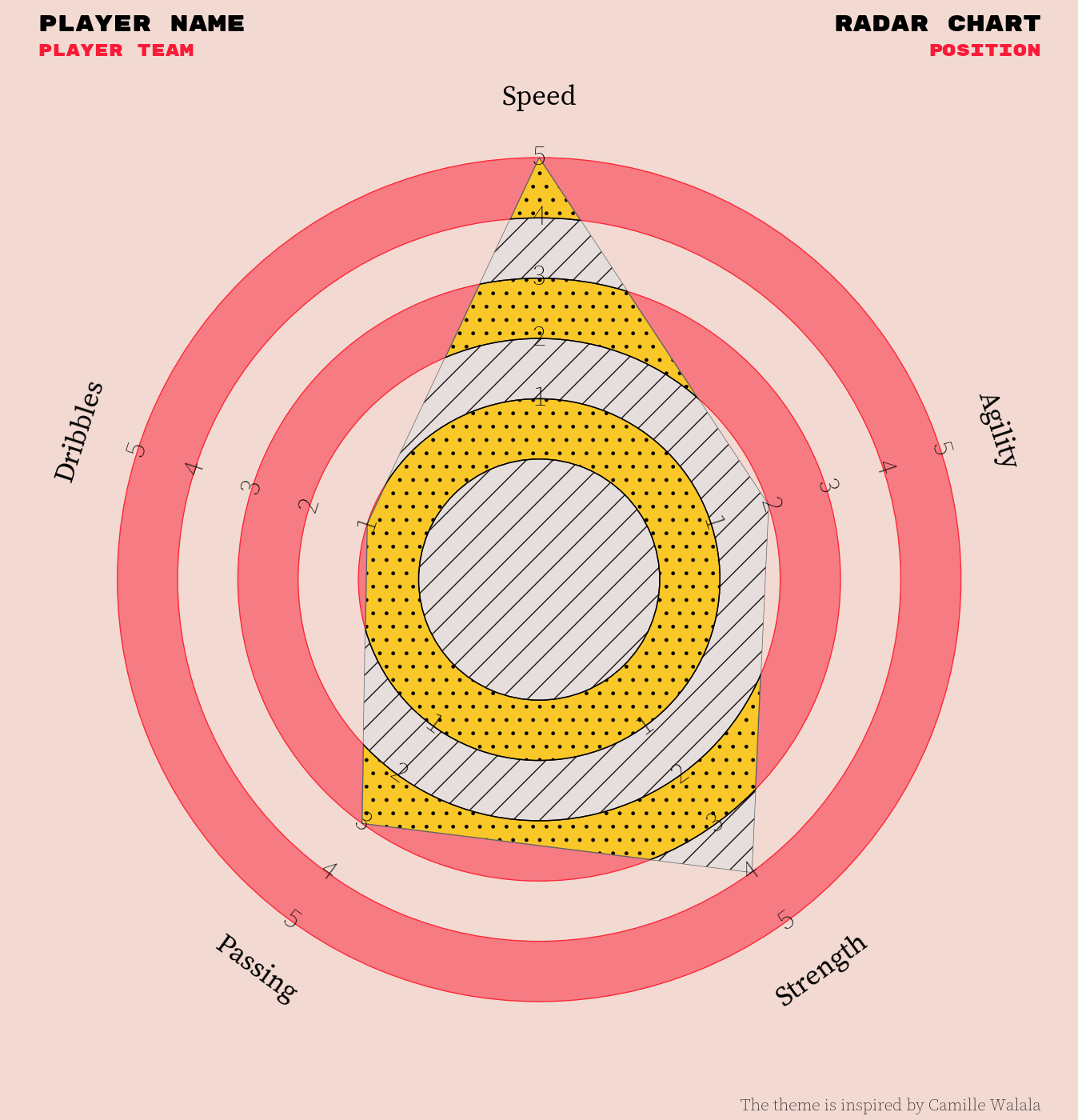
Camille Walala theme
The theme below is inspired by the London based artist Camille Walala. It uses two types of hatching to create the radar.
# creating the figure using the grid function from mplsoccer:
fig, axs = grid(figheight=14, grid_height=0.915, title_height=0.06, endnote_height=0.025,
                title_space=0, endnote_space=0, grid_key='radar', axis=False)

# we are creating a new radar object with more rings, integer rounding, and a larger center circle
radar2 = Radar(params=['Speed', 'Agility', 'Strength', 'Passing', 'Dribbles'],
               min_range=[0, 0, 0, 0, 0],
               max_range=[5, 5, 5, 5, 5],
               # here we make the labels integers instead of floats
               round_int=[True, True, True, True, True],
               # make the center circle x2 larger than the concentric circles
               center_circle_radius=2,
               # the number of rings has been chosen to divide the max_range evenly
               num_rings=5)

# plot the radar
radar2.setup_axis(ax=axs['radar'], facecolor='None')
rings_inner = radar2.draw_circles(ax=axs['radar'], facecolor='#f77b83', edgecolor='#fe2837')
radar_output = radar2.draw_radar(values=[5, 2, 4, 3, 1], ax=axs['radar'],
                                 kwargs_radar={'facecolor': '#f9c728', 'hatch': '.', 'alpha': 1},
                                 kwargs_rings={'facecolor': '#e6dedc', 'edgecolor': '#1a1414',
                                               'hatch': '/', 'alpha': 1})
# draw the radar again but without a facecolor ('None') and an edgecolor
# we draw it again so that we can choose a different edgecolor from the radar
radar_output2 = radar2.draw_radar(values=[5, 2, 4, 3, 1], ax=axs['radar'],
                                  kwargs_radar={'facecolor': 'None', 'edgecolor': '#646366'},
                                  kwargs_rings={'facecolor': 'None'})
# draw the labels
range_labels = radar2.draw_range_labels(ax=axs['radar'], fontproperties=serif_extra_light.prop,
                                        fontsize=25)
param_labels = radar2.draw_param_labels(ax=axs['radar'], fontproperties=serif_regular.prop,
                                        fontsize=25)

# adding the endnote and title text (these axes range from 0-1, i.e. 0, 0 is the bottom left)
# Note we are slightly offsetting the text from the edges by 0.01 (1%, e.g. 0.99)
endnote_text = axs['endnote'].text(0.99, 0.5, 'The theme is inspired by Camille Walala',
                                   fontproperties=serif_extra_light.prop, fontsize=15,
                                   ha='right', va='center')
title1_text = axs['title'].text(0.01, 0.65, 'Player name', fontsize=20,
                                fontproperties=rubik_regular.prop, ha='left', va='center')
title2_text = axs['title'].text(0.01, 0.25, 'Player team', fontsize=15,
                                fontproperties=rubik_regular.prop, ha='left',
                                va='center', color='#fa1b38')
title3_text = axs['title'].text(0.99, 0.65, 'Radar Chart', fontsize=20,
                                fontproperties=rubik_regular.prop, ha='right', va='center')
title4_text = axs['title'].text(0.99, 0.25, 'Position', fontsize=15,
                                fontproperties=rubik_regular.prop, ha='right',
                                va='center', color='#fa1b38')

fig.set_facecolor('#f2dad2')

plt.show()  # If you are using a Jupyter notebook you do not need this line
Total running time of the script: (0 minutes 2.847 seconds)