Note
Go to the end to download the full example code.
Improvements to expected threat
This example tries to make some improvements to our Expected threat model. Such as filtering out set pieces, changing the grid layout, and changing the simple goal probabilities with the average of a better expected goals model. Can you think of any more improvements?
import matplotlib.patheffects as path_effects
import matplotlib.pyplot as plt
import numpy as np
import pandas as pd

from mplsoccer import Sbopen, Pitch

parser = Sbopen()
pitch = Pitch(line_zorder=2)
Set up the grid
Let’s switch our simple 16 by 12 grid to something closer to the positional play grid. Here we reduce the number of cells before the half way line to one in the x-direction.
bins = (pitch.dim.positional_x[[0, 3, 4, 5, 6]], pitch.dim.positional_y)
Get event data
Get event data from the FA Women’s Super League 2019/20. Here we exclude shots/moves from direct set pieces from the events.
# first let's get the match file which lists all the match identifiers for
# the 87 games from the FA WSL 2019/20
df_match = parser.match(competition_id=37, season_id=42)
match_ids = df_match.match_id.unique()

# next we create a dataframe of all the events
all_events_df = []
set_pieces = ['Throw-in', 'Free Kick', 'Goal Kick', 'Corner', 'Kick Off', 'Penalty']
cols = ['match_id', 'id', 'type_name', 'sub_type_name', 'player_name',
        'x', 'y', 'end_x', 'end_y', 'outcome_name', 'shot_statsbomb_xg']
for match_id in match_ids:
    # get carries/ passes/ shots
    event = parser.event(match_id)[0]  # get the first dataframe (events) which has index = 0
    event = event.loc[((event.type_name.isin(['Carry', 'Shot', 'Pass'])) &
                       (~event['sub_type_name'].isin(set_pieces))),  # remove set-piece events
                      cols].copy()

    # boolean columns for working out probabilities
    event['goal'] = event['outcome_name'] == 'Goal'
    event['shoot'] = event['type_name'] == 'Shot'
    event['move'] = event['type_name'] != 'Shot'
    all_events_df.append(event)
event = pd.concat(all_events_df)
Bin the data
We make one change and average the expected goal results instead of using the raw goal probabilities in each grid cell.
shot_probability = pitch.bin_statistic(event['x'], event['y'], values=event['shoot'],
                                       statistic='mean', bins=bins)
move_probability = pitch.bin_statistic(event['x'], event['y'], values=event['move'],
                                       statistic='mean', bins=bins)
goal_probability = pitch.bin_statistic(event.loc[event['shoot'], 'x'],
                                       event.loc[event['shoot'], 'y'],
                                       event.loc[event['shoot'], 'shot_statsbomb_xg'],
                                       statistic='mean',
                                       bins=bins)
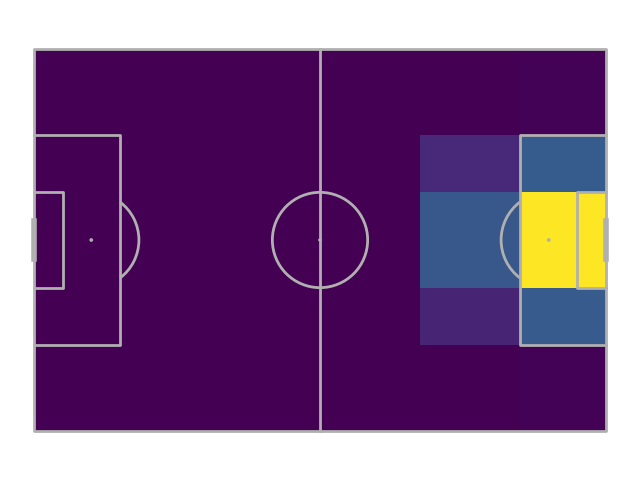
Plot shot probability
fig, ax = pitch.draw()
shot_heatmap = pitch.heatmap(shot_probability, ax=ax)
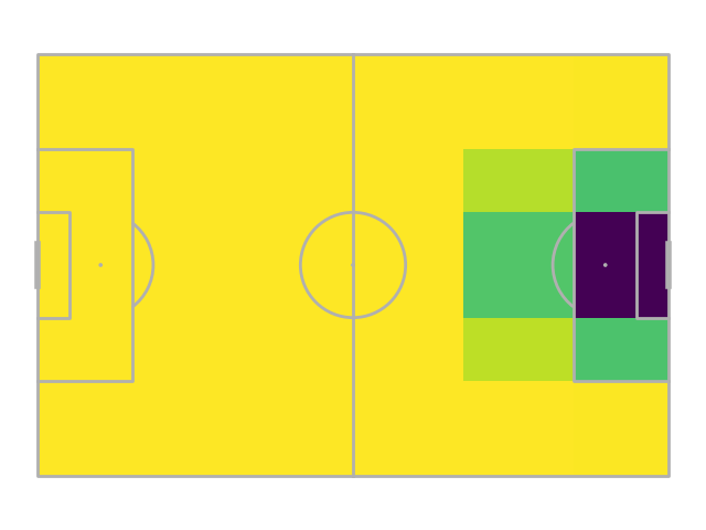
Plot move probability
fig, ax = pitch.draw()
move_heatmap = pitch.heatmap(move_probability, ax=ax)
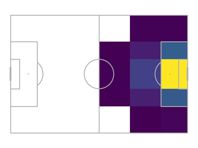
Plot goal probability
Notice here that the probabilities are far smoother than before, particular from areas such as the corners where it is rarer to shoot.
fig, ax = pitch.draw()
goal_heatmap = pitch.heatmap(goal_probability, ax=ax)
Calculate the move transition matrix
We keep the code the same for creating the move transition matrix.
# get a dataframe of move events and filter it
# so the dataframe only contains actions inside the pitch.
move = event[event['move']].copy()
bin_start_locations = pitch.bin_statistic(move['x'], move['y'], bins=bins)
move = move[bin_start_locations['inside']].copy()

# get the successful moves, which filters out the events that ended outside the pitch
# or where not successful (null)
bin_end_locations = pitch.bin_statistic(move['end_x'], move['end_y'], bins=bins)
move_success = move[(bin_end_locations['inside']) & (move['outcome_name'].isnull())].copy()

# get a dataframe of the successful moves
# and the grid cells they started and ended in
bin_success_start = pitch.bin_statistic(move_success['x'], move_success['y'], bins=bins)
bin_success_end = pitch.bin_statistic(move_success['end_x'], move_success['end_y'], bins=bins)
df_bin = pd.DataFrame({'x': bin_success_start['binnumber'][0],
                       'y': bin_success_start['binnumber'][1],
                       'end_x': bin_success_end['binnumber'][0],
                       'end_y': bin_success_end['binnumber'][1]})

# calculate the bin counts for the successful moves, i.e. the number of moves between grid cells
bin_counts = df_bin.value_counts().reset_index(name='bin_counts')

# create the move_transition_matrix of shape (num_y_bins, num_x_bins, num_y_bins, num_x_bins)
# this is the number of successful moves between grid cells.
num_y, num_x = shot_probability['statistic'].shape
move_transition_matrix = np.zeros((num_y, num_x, num_y, num_x))
move_transition_matrix[bin_counts['y'], bin_counts['x'],
                       bin_counts['end_y'], bin_counts['end_x']] = bin_counts.bin_counts.values

# and divide by the starting locations for all moves (including unsuccessful)
# to get the probability of moving the ball successfully between grid cells
bin_start_locations = pitch.bin_statistic(move['x'], move['y'], bins=bins)
bin_start_locations = np.expand_dims(bin_start_locations['statistic'], (2, 3))
move_transition_matrix = np.divide(move_transition_matrix,
                                   bin_start_locations,
                                   out=np.zeros_like(move_transition_matrix),
                                   where=bin_start_locations != 0,
                                   )
Get the matrices
move_transition_matrix = np.nan_to_num(move_transition_matrix)
shot_probability_matrix = np.nan_to_num(shot_probability['statistic'])
move_probability_matrix = np.nan_to_num(move_probability['statistic'])
goal_probability_matrix = np.nan_to_num(goal_probability['statistic'])
Calculate xT
xt = np.multiply(shot_probability_matrix, goal_probability_matrix)
diff = 1
iteration = 0
while np.any(diff > 0.00001):  # iterate until the differences between the old and new xT is small
    xt_copy = xt.copy()  # keep a copy for comparing the differences
    # calculate the new expected threat
    xt = (np.multiply(shot_probability_matrix, goal_probability_matrix) +
          np.multiply(move_probability_matrix,
                      np.multiply(move_transition_matrix, np.expand_dims(xt, axis=(0, 1))).sum(
                          axis=(2, 3)))
          )
    diff = (xt - xt_copy)
    iteration += 1
print('Number of iterations:', iteration)
Number of iterations: 35
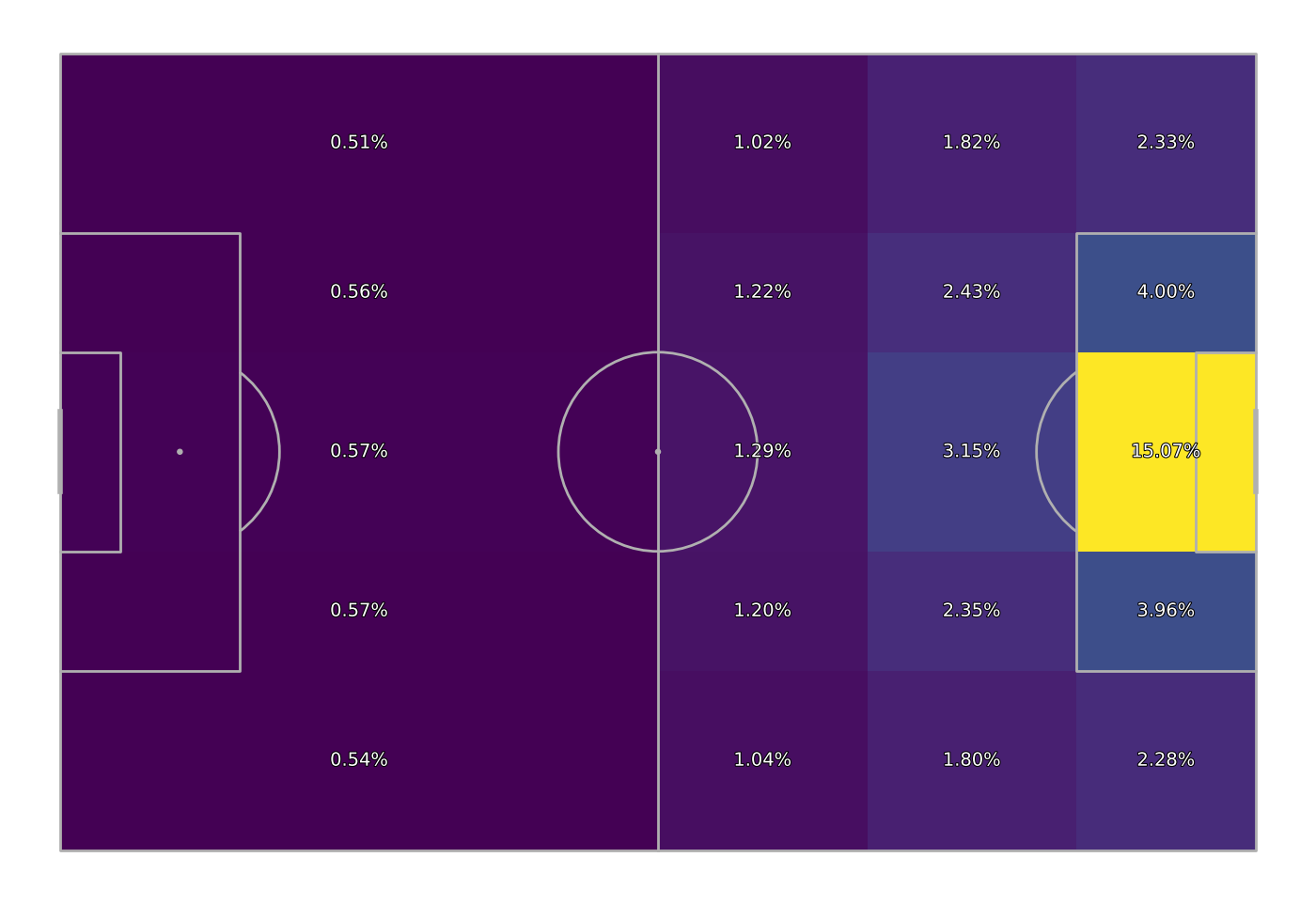
Plot xT grid
Plot the xT grid
path_eff = [path_effects.Stroke(linewidth=1.5, foreground='black'),
            path_effects.Normal()]
# new bin statistic for plotting xt only
for_plotting = pitch.bin_statistic(event['x'], event['y'], bins=bins)
for_plotting['statistic'] = xt
fig, ax = pitch.draw(figsize=(14, 9.625))
_ = pitch.heatmap(for_plotting, ax=ax)
_ = pitch.label_heatmap(for_plotting, ax=ax, str_format='{:.2%}',
                        color='white', fontsize=14, va='center', ha='center',
                        path_effects=path_eff)
# sphinx_gallery_thumbnail_path = 'gallery/tutorials/images/sphx_glr_plot_xt_improvements_004'
Scoring events
We score each successful move as the additional expected threat gained from moving from one grid cell to another grid cell.
# first get grid start and end cells
grid_start = pitch.bin_statistic(move_success.x, move_success.y, bins=bins)
grid_end = pitch.bin_statistic(move_success.end_x, move_success.end_y, bins=bins)

# then get the xT values from the start and end grid cell
start_xt = xt[grid_start['binnumber'][1], grid_start['binnumber'][0]]
end_xt = xt[grid_end['binnumber'][1], grid_end['binnumber'][0]]

# then calculate the added xT
added_xt = end_xt - start_xt
move_success['xt'] = added_xt

# show players with top 5 total expected threat
move_success.groupby('player_name')['xt'].sum().sort_values(ascending=False).head(5)
player_name
Janine Elizabeth Beckie          4.971296
Lisa Evans                       3.522066
Leah Galton                      3.329972
Jonna Ann-Charlotte Andersson    2.983019
Vivianne Miedema                 2.873153
Name: xt, dtype: float64
Wrap-up
We built a replica of the expected threat model Karun Singh used in his blog post, which has routes in Sarah Rudd work on using Markov models to value possession. We then tried out a few potential improvements. Now it’s over to you to try and build on this work.
plt.show() # If you are using a Jupyter notebook you do not need this line
Total running time of the script: (0 minutes 20.663 seconds)