Expected threat

This example shows how to create an expected threat (xT) model. Expected threat is a method for valuing the likelihood of scoring with possession of the ball at a position on the football pitch.

Expected threat is based on Markov chains. The main assumption for modelling soccer in this way is the probability of scoring only depends on the current action, it is memoryless, and it does not consider what happened before or after the event. Often in soccer, this isn’t a fair assumption as attacks may form quickly on the counter or due to pressuring the opponent high up the field. In reality how an action came about and how the defence is shifted may have an impact on what happens next.

I recommend reading through this excellent blog post by David Sumpter (@soccermatics) on the history of expected threat, its limitations, and possible extensions.

The first use of Markov chains to evaluate the probability of scoring was by Sarah Rudd in their conference presentation “a framework for tactical analysis and individual offensive production assessment in soccer using Markov chains.” Although not named expected threat it contained many of the ideas used here. Karun Singh then popularised and named the idea in their fantastic interactive blog post. In this tutorial, we model expected threat using Karun’s ideas in the blog post.

import matplotlib.patheffects as path_effects
import matplotlib.pyplot as plt
import numpy as np
import pandas as pd

from mplsoccer import Sbopen, Pitch

parser = Sbopen()
pitch = Pitch(line_zorder=2)

Set up the grid

Our first decision, is how to grid the soccer field. Here we copy Karun’s setup and have 16 cells in the x-direction and 12 cells in the y-direction

bins = (16, 12)  # 16 cells x 12 cells

Get event data

Get event data from the FA Women’s Super League 2019/20. Here we include only the carries, shots, and passes used to model expected threat. You may additionally want to filter out set pieces and counter-attacks.

# first let's get the match file which lists all the match identifiers for
# the 87 games from the FA WSL 2019/20
df_match = parser.match(competition_id=37, season_id=42)
match_ids = df_match.match_id.unique()

# next we create a dataframe of all the events
all_events_df = []
cols = ['match_id', 'id', 'type_name', 'sub_type_name', 'player_name',
        'x', 'y', 'end_x', 'end_y', 'outcome_name', 'shot_statsbomb_xg']
for match_id in match_ids:
    # get carries/ passes/ shots
    event = parser.event(match_id)[0]  # get the first dataframe (events) which has index = 0
    event = event.loc[event.type_name.isin(['Carry', 'Shot', 'Pass']), cols].copy()

    # boolean columns for working out probabilities
    event['goal'] = event['outcome_name'] == 'Goal'
    event['shoot'] = event['type_name'] == 'Shot'
    event['move'] = event['type_name'] != 'Shot'
    all_events_df.append(event)
event = pd.concat(all_events_df)

Bin the data

Here we calculate the probability of a shot, successful move (pass or carry), and goal (given a shot). We are averaging the boolean columns (True = 1) and (False = 0) to give us the probability between zero and one.

shot_probability = pitch.bin_statistic(event['x'], event['y'], values=event['shoot'],
                                       statistic='mean', bins=bins)
move_probability = pitch.bin_statistic(event['x'], event['y'], values=event['move'],
                                       statistic='mean', bins=bins)
goal_probability = pitch.bin_statistic(event.loc[event['shoot'], 'x'],
                                       event.loc[event['shoot'], 'y'],
                                       event.loc[event['shoot'], 'goal'],
                                       statistic='mean', bins=bins)

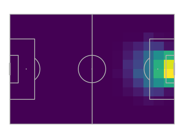
Plot shot probability

fig, ax = pitch.draw()
shot_heatmap = pitch.heatmap(shot_probability, ax=ax)

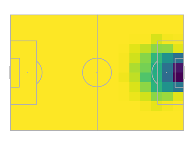
Plot move probability

As we only consider moves and shot probabilities. This is the mirror of the shot probability. The shot_probability + goal_probability adds up to one for each grid cell, as we assume only these two event types occur when in possession.

fig, ax = pitch.draw()
move_heatmap = pitch.heatmap(move_probability, ax=ax)

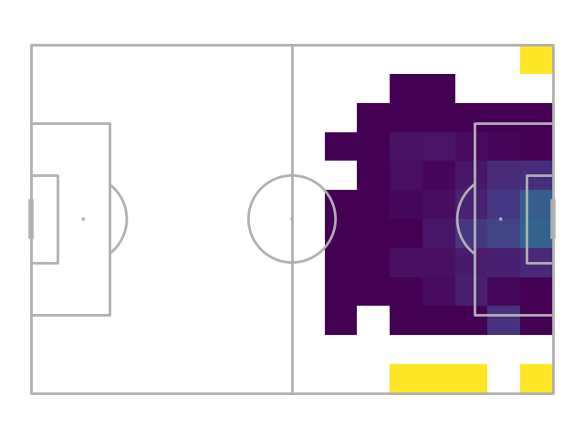
Plot goal probability

fig, ax = pitch.draw()
goal_heatmap = pitch.heatmap(goal_probability, ax=ax)

Calculate the move transition matrix

The move transition matrix takes into account the success probability of carrying out the transitions. It is the probability of moving the ball successfully from one grid cell to another grid cell.

# get a dataframe of move events and filter it
# so the dataframe only contains actions inside the pitch.
move = event[event['move']].copy()
bin_start_locations = pitch.bin_statistic(move['x'], move['y'], bins=bins)
move = move[bin_start_locations['inside']].copy()

# get the successful moves, which filters out the events that ended outside the pitch
# or where not successful (null)
bin_end_locations = pitch.bin_statistic(move['end_x'], move['end_y'], bins=bins)
move_success = move[(bin_end_locations['inside']) & (move['outcome_name'].isnull())].copy()

# get a dataframe of the successful moves
# and the grid cells they started and ended in
bin_success_start = pitch.bin_statistic(move_success['x'], move_success['y'], bins=bins)
bin_success_end = pitch.bin_statistic(move_success['end_x'], move_success['end_y'], bins=bins)
df_bin = pd.DataFrame({'x': bin_success_start['binnumber'][0],
                       'y': bin_success_start['binnumber'][1],
                       'end_x': bin_success_end['binnumber'][0],
                       'end_y': bin_success_end['binnumber'][1]})

# calculate the bin counts for the successful moves, i.e. the number of moves between grid cells
bin_counts = df_bin.value_counts().reset_index(name='bin_counts')

# create the move_transition_matrix of shape (num_y_bins, num_x_bins, num_y_bins, num_x_bins)
# this is the number of successful moves between grid cells.
num_y, num_x = shot_probability['statistic'].shape
move_transition_matrix = np.zeros((num_y, num_x, num_y, num_x))
move_transition_matrix[bin_counts['y'], bin_counts['x'],
                       bin_counts['end_y'], bin_counts['end_x']] = bin_counts.bin_counts.values

# and divide by the starting locations for all moves (including unsuccessful)
# to get the probability of moving the ball successfully between grid cells
bin_start_locations = pitch.bin_statistic(move['x'], move['y'], bins=bins)
bin_start_locations = np.expand_dims(bin_start_locations['statistic'], (2, 3))
move_transition_matrix = np.divide(move_transition_matrix,
                                   bin_start_locations,
                                   out=np.zeros_like(move_transition_matrix),
                                   where=bin_start_locations != 0,
                                   )

Get the matrices

Get the matrices from the dictionaries and turn nans into zeros

move_transition_matrix = np.nan_to_num(move_transition_matrix)
shot_probability_matrix = np.nan_to_num(shot_probability['statistic'])
move_probability_matrix = np.nan_to_num(move_probability['statistic'])
goal_probability_matrix = np.nan_to_num(goal_probability['statistic'])

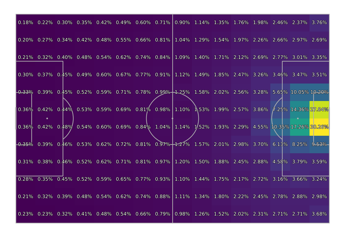
Calculate xT

Calculate xT until convergence. Initially the expected threat is set to the shot probability multiplied by the goal probability. This means the expected value in the first step is the probability of scoring from the grid cell if the person takes a shot.

xt = np.multiply(shot_probability_matrix, goal_probability_matrix)
diff = 1
iteration = 0
while np.any(diff > 0.00001):  # iterate until the differences between the old and new xT is small
    xt_copy = xt.copy()  # keep a copy for comparing the differences
    # calculate the new expected threat
    xt = (np.multiply(shot_probability_matrix, goal_probability_matrix) +
          np.multiply(move_probability_matrix,
                      np.multiply(move_transition_matrix, np.expand_dims(xt, axis=(0, 1))).sum(
                          axis=(2, 3)))
          )
    diff = (xt - xt_copy)
    iteration += 1
print('Number of iterations:', iteration)

Number of iterations: 36

Plot xT grid

Plot the xT grid

path_eff = [path_effects.Stroke(linewidth=1.5, foreground='black'),
            path_effects.Normal()]
# new bin statistic for plotting xt only
for_plotting = pitch.bin_statistic(event['x'], event['y'], bins=bins)
for_plotting['statistic'] = xt
fig, ax = pitch.draw(figsize=(14, 9.625))
_ = pitch.heatmap(for_plotting, ax=ax)
_ = pitch.label_heatmap(for_plotting, ax=ax, str_format='{:.2%}',
                        color='white', fontsize=14, va='center', ha='center',
                        path_effects=path_eff)
# sphinx_gallery_thumbnail_path = 'gallery/tutorials/images/sphx_glr_plot_xt_004'

Scoring events

We score each successful move as the additional expected threat gained from moving from one grid cell to another grid cell.

# first get grid start and end cells
grid_start = pitch.bin_statistic(move_success.x, move_success.y, bins=bins)
grid_end = pitch.bin_statistic(move_success.end_x, move_success.end_y, bins=bins)

# then get the xT values from the start and end grid cell
start_xt = xt[grid_start['binnumber'][1], grid_start['binnumber'][0]]
end_xt = xt[grid_end['binnumber'][1], grid_end['binnumber'][0]]

# then calculate the added xT
added_xt = end_xt - start_xt
move_success['xt'] = added_xt

# show players with top 5 total expected threat
move_success.groupby('player_name')['xt'].sum().sort_values(ascending=False).head(5)

player_name
Caroline Weir              7.201262
Guro Reiten                6.966561
Fara Williams              5.752318
Janine Elizabeth Beckie    5.687048
Lisa Evans                 4.285504
Name: xt, dtype: float64

Improvements

Now we have a simple model, let’s try to make some Improvements to expected threat model.

plt.show()  # If you are using a Jupyter notebook you do not need this line