Bin Statistic Sonar

StatsBomb has a great blog on the history of Sonars. Sonars show more information than heatmaps by introducing the angle of passes, shots or other events.

The following examples show how to use the bin_statistic_sonar method to bin data by x/y coordinates and angles. More information is available on how to customize the plotted sonars in Sonar Grid and Sonar.

import matplotlib.pyplot as plt
import numpy as np

from mplsoccer import Pitch, VerticalPitch, Sbopen

Load the first game that Messi played as a false-9.

parser = Sbopen()
df = parser.event(69249)[0]  # 0 index is the event file
df = df[(df.type_name == 'Pass') & (df.team_name == 'Barcelona') &
        (~df.sub_type_name.isin(['Free Kick', 'Throw-in',
                                 'Goal Kick', 'Kick Off', 'Corner']))].copy()

Plot a Pass Sonar

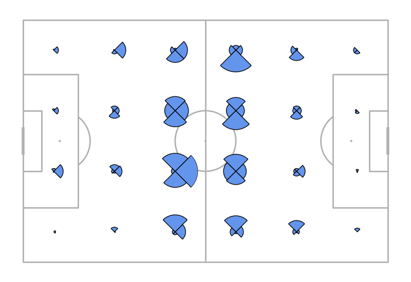
Here, we calculate the angle and distance for each pass. We then split the data into 6x4 grid cells. Within each grid cell, we split the data into four equal segments of 90 degrees (360 / 4). The defaults count the number of actions (passes) in each segment.

pitch = Pitch()
angle, distance = pitch.calculate_angle_and_distance(df.x, df.y, df.end_x, df.end_y)
bs = pitch.bin_statistic_sonar(df.x, df.y, angle,
                               bins=(6, 4, 4),  # x, y, angle binning
                               # center the first angle so it starts
                               # at -45 degrees (90 / 2) rather than 0 degrees
                               center=True)
fig, ax = pitch.draw(figsize=(8, 5.5))
axs = pitch.sonar_grid(bs, width=15, fc='cornflowerblue', ec='black', ax=ax)

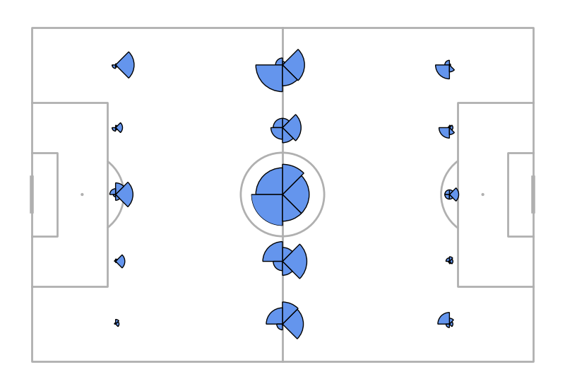
Center argument

You can either center the first slice around zero degrees (center=True) or start the first segment at zero degrees (center=False).

pitch = VerticalPitch()
fig, axs = pitch.draw(figsize=(8, 6), nrows=1, ncols=2)
angle, distance = pitch.calculate_angle_and_distance(df.x, df.y, df.end_x, df.end_y)
bs_center = pitch.bin_statistic_sonar(df.x, df.y, angle, bins=(6, 4, 4), center=True)
bs_not_center = pitch.bin_statistic_sonar(df.x, df.y, angle, bins=(6, 4, 4), center=False)
axs_sonar = pitch.sonar_grid(bs_center, width=15, fc='cornflowerblue', ec='black', ax=axs[0])
axs_sonar = pitch.sonar_grid(bs_not_center, width=15, fc='cornflowerblue', ec='black', ax=axs[1])
text1 = pitch.text(60, 40, 'center=True', va='center', ha='center', fontsize=15, ax=axs[0])
text1 = pitch.text(60, 40, 'center=False', va='center', ha='center', fontsize=15, ax=axs[1])

Statistic

The default statistic='count' calculates counts in each segment. You can also use the statistic and values arguments to calculate other statistics. Here, we calculate the average pass distance and plot this instead of the count of passes. You can also normalize results between 0 to 1 with the normalize=True argument.

pitch = Pitch()
angle, distance = pitch.calculate_angle_and_distance(df.x, df.y, df.end_x, df.end_y)
bs = pitch.bin_statistic_sonar(df.x, df.y, angle,
                               # calculate the average distance
                               # you can also calculate other statistics
                               # such as std, median, sum, min and the max
                               values=distance, statistic='mean',
                               bins=(6, 4, 4), center=True)
fig, ax = pitch.draw(figsize=(8, 5.5))
axs = pitch.sonar_grid(bs, width=15, fc='cornflowerblue', ec='black', ax=ax)

Bins

In addition to integer values for bins, you can use a sequence of angle edges. The angle edges should be between zero and 2*pi (~6.283), i.e. the angles in radians. You can convert from degrees to radians using numpy.radians.

pitch = Pitch()
angle, distance = pitch.calculate_angle_and_distance(df.x, df.y, df.end_x, df.end_y)
x_bin = 3  # the bin argument can contain a mix of sequences and integers
y_bin = pitch.dim.positional_y
# I use cumsum so I can use widths rather than bin edges.
# I convert to radians using numpy
angle_bin = np.radians(np.array([0, 90, 45, 90, 90, 45])).cumsum()
bs = pitch.bin_statistic_sonar(df.x, df.y, angle,
                               bins=(x_bin, y_bin, angle_bin), center=True)
fig, ax = pitch.draw(figsize=(8, 5.5))
axs = pitch.sonar_grid(bs, width=15, fc='cornflowerblue', ec='black', ax=ax)

Binnumber

You can also get the bin numbers from the bin_statistic_sonar result. Here, we use the binnumber to filter for the forward passes in the final third and plot them as arrows.

pitch = Pitch()
angle, distance = pitch.calculate_angle_and_distance(df.x, df.y, df.end_x, df.end_y)
bs = pitch.bin_statistic_sonar(df.x, df.y, angle,
                               bins=(3, 1, 2), center=True)
fig, ax = pitch.draw(figsize=(8, 5.5))
axs = pitch.sonar_grid(bs, width=15, fc='cornflowerblue', ec='black', ax=ax)
mask = np.logical_and(np.logical_and(bs['binnumber'][0] == 2,  # x in the final third
                                     bs['binnumber'][1] == 0),
                      # only one y but here for completeness
                      bs['binnumber'][2] == 0  # first angle
                      )
arr = pitch.arrows(df[mask].x, df[mask].y, df[mask].end_x, df[mask].end_y, ax=ax)

plt.show()  # If you are using a Jupyter notebook you do not need this line