Turbine Charts

Here we jazz up radar charts by putting the distributions inside the radar chart. You can mix and match the various elements of the Radar class to create your own version.

Each blade of the turbine represents the statistics for the skill. While the blade is split at the point of the individual player’s skill level.

If you like this idea follow Soumyajit Bose on Twitter, as I borrowed some of his ideas for this chart.

import pandas as pd
from mplsoccer import Radar, FontManager, grid
import numpy as np
import scipy.stats as stats
import matplotlib.pyplot as plt

Creating some random data

Here we create some random data from a truncated normal distribution. In real life, the values would be an array or dataframe of shape number of players * number of skills

lower, upper, mu, sigma = 0, 1, 0.35, 0.25
X = stats.truncnorm((lower - mu) / sigma, (upper - mu) / sigma, loc=mu, scale=sigma)
# for 1000 people and 11 skills
values = X.rvs((1000, 11))
# the names of the skills
params = ['Expected goals', 'Total shots',
          'Touches in attacking penalty area', 'Pass completion %',
          'Crosses into the 18-yard box (excluding set pieces)',
          'Expected goals assisted', 'Fouls drawn', 'Successful dribbles',
          'Successful pressures', 'Non-penalty expected goals per shot',
          'Miscontrols/ Dispossessed']
# set up a dataframe with the random values
df = pd.DataFrame(values)
df.columns = params
# in real-life you'd probably have a string column for the player name,
# but we will use numbers here
df['player_name'] = np.arange(1000)

Instantiate the Radar Class

We will instantiate a radar object and set the lower and upper bounds. For miscontrols/ dispossessed it is better to have a lower number, so we will flip the statistic by adding the parameter to lower_is_better.

# create the radar object with an upper and lower bound of the 5% and 95% quantiles
low = df[params].quantile(0.05).values
high = df[params].quantile(0.95).values
lower_is_better = ['Miscontrols/ Dispossessed']
radar = Radar(params, low, high, lower_is_better=lower_is_better, num_rings=4)

Load a font

We will use mplsoccer’s FontManager to load the default Robotto font.

fm = FontManager()

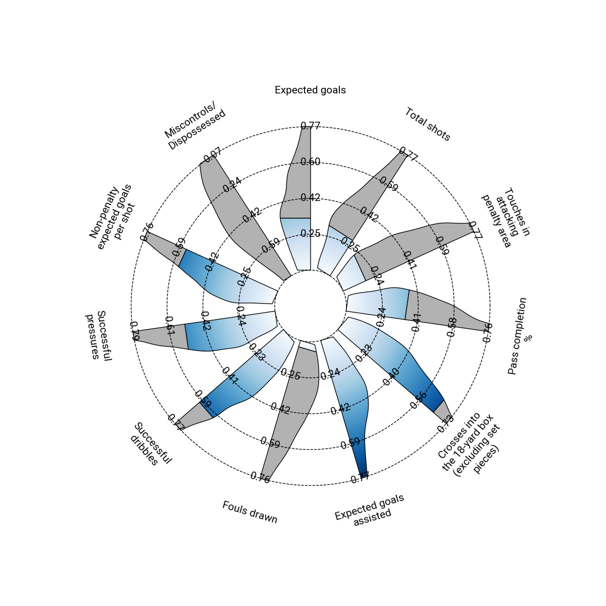
Making a Simple Turbine Chart

Here we will make a very simple turbine chart using the radar_chart module.

# get the player's values (usually the 23 would be a string)
# so for example you might put
# df.loc[df.player_name == 'Martin Ødegaard', params].values[0].tolist()
player_values = df.loc[df.player_name == 23, params].values[0]

# plot the turbine plot
fig, ax = radar.setup_axis()  # format axis as a radar
# plot the turbine blades. Here we give the player_Values and the
# value for all players shape=(1000, 11)
turbine_output = radar.turbine(player_values, df[params].values, ax=ax,
                               kwargs_inner={'edgecolor': 'black'},
                               kwargs_inner_gradient={'cmap': 'Blues'},
                               kwargs_outer={'facecolor': '#b2b2b2', 'edgecolor': 'black'})
# plot some dashed rings and the labels for the values and parameter names
rings_inner = radar.draw_circles(ax=ax, facecolor='None', edgecolor='black', linestyle='--')
range_labels = radar.draw_range_labels(ax=ax, fontsize=15, fontproperties=fm.prop, zorder=2)
param_labels = radar.draw_param_labels(ax=ax, fontsize=15, fontproperties=fm.prop, zorder=2)

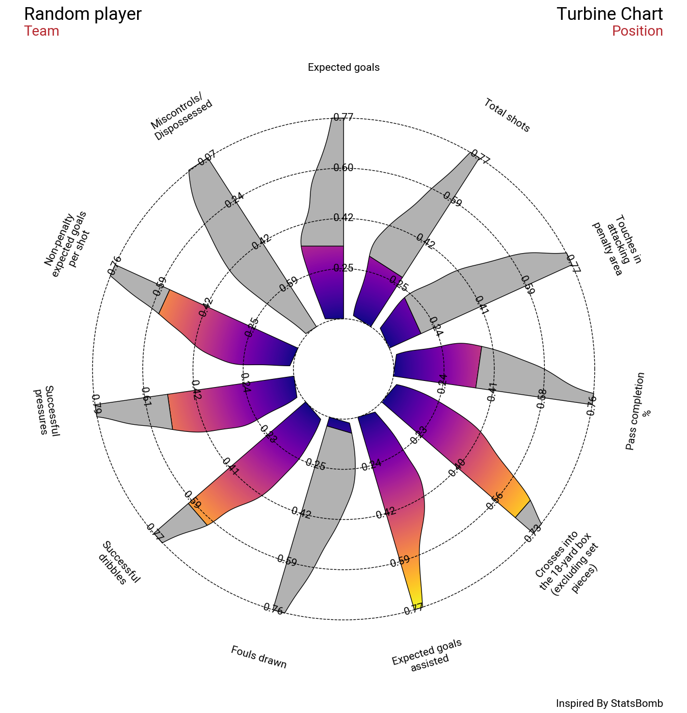
Adding a title and endnote

Here we will add an endnote and title to the Radar. We will use the grid function to create the figure and pass the axs[‘radar’] axes to the Radar’s methods.

# creating the figure using the grid function from mplsoccer:
fig, axs = grid(figheight=14, grid_height=0.915, title_height=0.06, endnote_height=0.025,
                title_space=0, endnote_space=0, grid_key='radar', axis=False)

# plot the turbine plot
radar.setup_axis(ax=axs['radar'])
# plot the turbine blades. Here we give the player_Values and
# the value for all players shape=(1000, 11)
turbine_output = radar.turbine(player_values, df[params].values, ax=axs['radar'],
                               kwargs_inner={'edgecolor': 'black'},
                               kwargs_inner_gradient={'cmap': 'plasma'},
                               kwargs_outer={'facecolor': '#b2b2b2', 'edgecolor': 'black'})
# plot some dashed rings and the labels for the values and parameter names
rings_inner = radar.draw_circles(ax=axs['radar'], facecolor='None',
                                 edgecolor='black', linestyle='--')
range_labels = radar.draw_range_labels(ax=axs['radar'], fontsize=15,
                                       fontproperties=fm.prop, zorder=2)
param_labels = radar.draw_param_labels(ax=axs['radar'], fontsize=15,
                                       fontproperties=fm.prop, zorder=2)

# adding a title and endnote
title1_text = axs['title'].text(0.01, 0.65, 'Random player', fontsize=25,
                                fontproperties=fm.prop, ha='left', va='center')
title2_text = axs['title'].text(0.01, 0.25, 'Team', fontsize=20,
                                fontproperties=fm.prop,
                                ha='left', va='center', color='#B6282F')
title3_text = axs['title'].text(0.99, 0.65, 'Turbine Chart', fontsize=25,
                                fontproperties=fm.prop, ha='right', va='center')
title4_text = axs['title'].text(0.99, 0.25, 'Position', fontsize=20,
                                fontproperties=fm.prop,
                                ha='right', va='center', color='#B6282F')
endnote_text = axs['endnote'].text(0.99, 0.5, 'Inspired By StatsBomb', fontsize=15,
                                   fontproperties=fm.prop, ha='right', va='center')

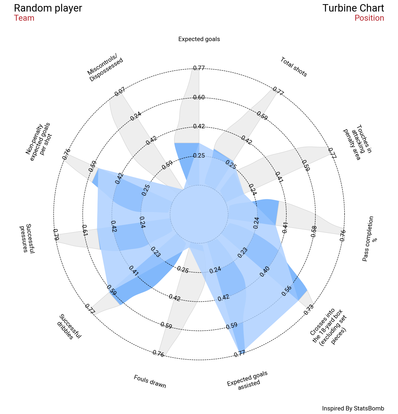
Mixing with Radars

You can also mix and match the different elements of Radars and Turbines.

# creating the figure using the grid function from mplsoccer:
fig, axs = grid(figheight=14, grid_height=0.915, title_height=0.06, endnote_height=0.025,
                title_space=0, endnote_space=0, grid_key='radar', axis=False)

# plot the turbine plot
radar.setup_axis(ax=axs['radar'])
# plot the turbine blades. Here we give the player_Values and
# the value for all players shape=(1000, 11)
turbine_output = radar.turbine(player_values, df[params].values, ax=axs['radar'],
                               kwargs_inner={'edgecolor': '#d4d4d4', 'color': '#81b8fb'},
                               kwargs_outer={'facecolor': '#eeeeee', 'edgecolor': '#d4d4d4'})
# plot some dashed rings and the labels for the values and parameter names
rings_inner = radar.draw_circles(ax=axs['radar'], facecolor='None',
                                 edgecolor='black', linestyle='--')
range_labels = radar.draw_range_labels(ax=axs['radar'], fontsize=15,
                                       fontproperties=fm.prop, zorder=12)
param_labels = radar.draw_param_labels(ax=axs['radar'], fontsize=15,
                                       fontproperties=fm.prop, zorder=2)
# overlay the radar
radar_output = radar.draw_radar(player_values, ax=axs['radar'],
                                kwargs_radar={'facecolor': '#9dc7ff', 'alpha': 0.7},
                                kwargs_rings={'facecolor': '#bbd8ff', 'alpha': 0.7})

# adding a title and endnote
title1_text = axs['title'].text(0.01, 0.65, 'Random player', fontsize=25,
                                fontproperties=fm.prop, ha='left', va='center')
title2_text = axs['title'].text(0.01, 0.25, 'Team', fontsize=20,
                                fontproperties=fm.prop,
                                ha='left', va='center', color='#B6282F')
title3_text = axs['title'].text(0.99, 0.65, 'Turbine Chart', fontsize=25,
                                fontproperties=fm.prop, ha='right', va='center')
title4_text = axs['title'].text(0.99, 0.25, 'Position', fontsize=20,
                                fontproperties=fm.prop,
                                ha='right', va='center', color='#B6282F')
endnote_text = axs['endnote'].text(0.99, 0.5, 'Inspired By StatsBomb', fontsize=15,
                                   fontproperties=fm.prop, ha='right', va='center')

plt.show()  # not needed in Jupyter notebooks